Molecular Dynamics Trajectory Quality Assessment: From Foundational Principles to Advanced Validation in Biomedical Research
This comprehensive article explores current methodologies and best practices for assessing the quality of molecular dynamics (MD) trajectories, a critical challenge in computational biophysics and drug development.
Molecular Dynamics Trajectory Quality Assessment: From Foundational Principles to Advanced Validation in Biomedical Research
Abstract
This comprehensive article explores current methodologies and best practices for assessing the quality of molecular dynamics (MD) trajectories, a critical challenge in computational biophysics and drug development. As MD simulations become increasingly integral to understanding biological processes at atomic resolution, robust quality evaluation protocols are essential for ensuring reliable results. We examine foundational concepts of trajectory analysis, advanced methodological frameworks like the Quality Evaluation Based Simulation Selection (QEBSS) protocol, troubleshooting strategies for common pitfalls, and rigorous validation approaches comparing force fields and algorithms. Targeted at researchers, scientists, and drug development professionals, this review synthesizes recent advances from 2025 research to provide practical guidance for implementing effective trajectory quality assessment in biomedical applications, from protein dynamics studies to drug solubility prediction.
The Fundamentals of MD Trajectory Quality: Understanding Core Metrics and Their Biophysical Significance
Molecular Dynamics (MD) simulation has become an indispensable tool in structural biology, biophysics, and drug discovery, enabling researchers to investigate the dynamic evolution of biomolecular systems with exceptional detail [1]. The technique models physical system motions by solving dynamical equations of motion based on parameterized force fields, generating trajectories that depict conformational sampling over time [2]. However, the value of these simulations hinges on their quality and reliability, necessitating robust assessment methodologies. Within the broader context of molecular dynamics trajectory quality assessment research, this guide objectively compares the essential metrics used to evaluate simulation performance: Root Mean Square Deviation (RMSD), Root Mean Square Fluctuation (RMSF), Radius of Gyration (Rg), and energy conservation principles. These quantitative measures provide complementary insights into different aspects of trajectory quality, from global structural stability to local residue flexibility and system thermodynamics.
Core Quality Metrics Comparison
Definition and Applications of Key Metrics
MD simulations generate enormous amounts of trajectory data, and specific metrics have been standardized to evaluate different aspects of structural dynamics and simulation quality.
Root Mean Square Deviation (RMSD): This fundamental metric calculates the average distance between atoms of a protein or protein complex relative to a reference structure, typically the initial frame. RMSD primarily assesses structural stability, convergence of the simulation system, and the status of conformational changes over time [3]. It provides a global measure of how much the structure deviates from its starting configuration or other reference states.
Root Mean Square Fluctuation (RMSF): This residue-specific metric quantifies the average fluctuation of each residue relative to its mean position throughout the simulation trajectory. RMSF is particularly valuable for identifying flexible and rigid regions within a protein, illuminating domains with significant dynamic behavior that may be crucial for biological function [3].
Radius of Gyration (Rg): Rg measures the mean distance of atoms from the center of mass of a protein, providing insights into its overall compactness and folding state. Low Rg values depict a more compact structure (folded state), while high Rg values depict an expanded structure (unfolded state) [3]. This metric is especially useful for studying folding/unfolding processes and conformational compaction.
Energy Conservation: In microcanonical (NVE) ensemble simulations, the principle of energy conservation requires that the total energy of an isolated system remains constant over time. Monitoring the fluctuation of total energy provides a critical check on the stability and physical validity of the simulation, with significant energy drift indicating potential problems with the integration algorithm, force field parameters, or simulation setup.
Comparative Analysis of Metrics
Table 1: Comprehensive Comparison of Essential MD Quality Metrics
| Metric | Structural Level | Primary Application | Interpretation Guidelines | Computational Domain |
|---|---|---|---|---|
| RMSD | Global | Structural stability and convergence [3] | Low values indicate stable simulation; significant jumps may indicate conformational changes [4] | Backbone or Cα atoms typically used to eliminate noise from side chain motions |
| RMSF | Local (per-residue) | Flexibility and dynamics of residues [3] | High values indicate flexible regions; low values indicate rigid structural elements [5] | Cα atoms commonly analyzed to identify functionally important flexible regions |
| Rg | Global | Compactness and folding state [3] | Low values = compact/folded; high values = expanded/unfolded [3] | All atoms or backbone atoms to assess overall structural compaction |
| Energy Conservation | System-level | Physical validity and numerical stability [2] | Stable total energy = physically realistic; energy drift = potential integration problems | Total energy of the system monitored throughout production simulation |
Experimental Protocols and Methodologies
Standard MD Simulation Workflow
The assessment of quality metrics follows a standardized MD workflow that ensures proper system preparation, equilibration, and production phases:
System Preparation: The protein structure is obtained from experimental sources (Protein Data Bank) or computational modeling approaches such as AlphaFold2, Robetta-RoseTTAFold, or homology modeling [4] [6]. The structure is solvated in a water box (typically TIP3P water model) with ions added to neutralize the system and achieve physiological salt concentration (e.g., 0.15 M NaCl) [7].
Energy Minimization: The system undergoes energy minimization using algorithms like steepest descent until the maximum force is below a specified threshold (e.g., 1000 kJ/(mol·nm)) to remove steric clashes and bad contacts [7].
Equilibration: The minimized system undergoes equilibration in two phases:
- NVT equilibration (constant Number of particles, Volume, and Temperature) for 100 ps to stabilize the temperature at the target value (typically 310 K for biological systems) using thermostats like Berendsen [7].
- NPT equilibration (constant Number of particles, Pressure, and Temperature) for 100 ps to stabilize the pressure at 1.0 bar using barostats like Parrinello-Rahman [7].
Production Simulation: The equilibrated system proceeds to production MD simulation for data collection, typically ranging from 100 ns to 1 μs depending on the system size and research question. Trajectories are saved at regular intervals (e.g., every 10-100 ps) for subsequent analysis [7] [8].
Trajectory Analysis: The saved trajectories are analyzed using tools like GROMACS, VMD, or ProProtein to calculate quality metrics including RMSD, RMSF, Rg, and energy conservation [1].
Metric Calculation Protocols
Table 2: Detailed Methodologies for Calculating Essential Quality Metrics
| Metric | Calculation Method | Technical Parameters | Software Implementation | ||
|---|---|---|---|---|---|
| RMSD | RMSD = √(1/N × Σᵢ[(xᵢ - xᵢref)² + (yᵢ - yᵢref)² + (zᵢ - zᵢref)²]) where N is the number of atoms, (x,y,z) are coordinates, and (xref,yref,zref) are reference coordinates [2] | Typically calculated after rotational and translational fitting to reference structure; often using backbone or Cα atoms | GROMACS (gmx rms), VMD, ProProtein [1] |
||
| RMSF | RMSFᵢ = √(⟨(rᵢ - ⟨rᵢ⟩)²⟩) where rᵢ is the position of atom i, and ⟨⟩ denotes time average [2] | Calculated for each residue; requires prior fitting to remove global translation/rotation | GROMACS (gmx rmsf), ProProtein platform [1] |
||
| Rg | Rg = √(1/M × Σᵢ mᵢ(rᵢ - rcm)²) where M is total mass, mᵢ is mass of atom i, rᵢ is position, and rcm is center of mass [3] | Can be calculated for all atoms or specific subsets; often reported for backbone atoms | GROMACS (gmx gyrate), VMD |
||
| Energy Conservation | ΔE_total = | Etotal(t) - ⟨Etotal⟩ | / σE where Etotal is total energy, ⟨⟩ denotes average, and σ_E is standard deviation | Monitored throughout simulation; particularly critical for NVE ensembles | GROMACS (gmx energy), NAMD |
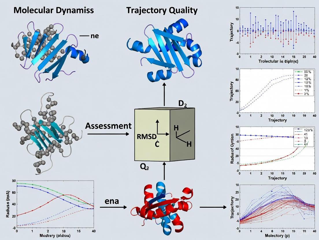
Figure 1: MD workflow and quality assessment metrics relationship. The diagram illustrates the standard molecular dynamics simulation workflow and its connection to the essential quality metrics used for trajectory validation.
The Scientist's Toolkit: Research Reagent Solutions
Table 3: Essential Software Tools and Computational Resources for MD Quality Assessment
| Tool/Resource | Type | Primary Function | Application in Quality Assessment |
|---|---|---|---|
| GROMACS | MD Software Suite | High-performance molecular dynamics simulations [7] [8] | Calculation of RMSD, RMSF, Rg, and energy monitoring through built-in analysis tools |
| ProProtein | Web Platform | Automated identification of 3D structure fluctuations in MD trajectories [1] | Visualization of high-fluctuation regions and trajectory quality assessment |
| CHARMM36 | Force Field | Parameterization of molecular interactions [7] | Provides physical basis for realistic simulation dynamics and energy conservation |
| AMBER99-SB-ILDN | Force Field | Alternative parameterization for biomolecular simulations [2] | Ensures accurate energy calculations and structural dynamics |
| GROMOS 54a7 | Force Field | Unified atom force field for MD simulations [8] | Parameterization for consistent energy conservation and structural properties |
| Visual Molecular Dynamics (VMD) | Visualization Software | Trajectory visualization and analysis [7] | Visual quality assessment and metric calculation through plugins |
| Molecular Operating Environment (MOE) | Modeling Software | Homology modeling and structure preparation [4] | Initial structure preparation and template-based modeling for simulation input |
The comprehensive assessment of molecular dynamics simulation quality requires the integrated application of multiple complementary metrics. RMSD provides essential information about global structural stability, RMSF reveals local flexibility patterns critical for functional mechanisms, Rg quantifies overall compactness and folding state, and energy conservation validates the physical realism of the simulation. Current research indicates that these metrics should not be considered in isolation but rather as an interconnected framework for trajectory validation [3] [2]. As MD simulations continue to advance in temporal and spatial complexity, with studies now routinely reaching microsecond timescales and investigating larger biomolecular assemblies [1], the rigorous application of these quality metrics becomes increasingly crucial for distinguishing physically meaningful results from computational artifacts. The development of automated platforms like ProProtein [1] represents the growing recognition that standardized, accessible quality assessment is fundamental to the continued advancement of molecular dynamics as a predictive tool in structural biology and drug discovery.
Spin relaxation measurements, specifically of the parameters T1 (longitudinal relaxation time), T2 (transverse relaxation time), and heteronuclear Nuclear Overhauser Effect (hetNOE), provide indispensable experimental windows into molecular dynamics at atomic resolution. These NMR parameters are sensitive to molecular motions because nuclear spin relaxation is mediated by fluctuating local magnetic fields caused by both the overall tumbling and internal movements of molecules [9]. For protein studies, backbone 15N relaxation serves as a primary experimental probe, reporting on dynamics across an extraordinary range of timescales from picoseconds to milliseconds [10]. The connection between these measurable parameters and underlying molecular motions is encoded in the spectral density function, J(ω), which describes the distribution of motional frequencies within the molecule [9] [11].
The interpretation of T1, T2, and hetNOE data enables researchers to characterize both the global rotational diffusion of biomolecules and site-specific internal flexibility, information crucial for understanding how structural dynamics relate to biological function. This guide systematically compares the predominant analytical frameworks used to extract motional information from relaxation data, assessing their theoretical foundations, practical implementations, and respective strengths in connecting NMR measurements to molecular dynamics.
Theoretical Foundations: From NMR Parameters to Molecular Motions
Fundamental Relationships
The core theoretical framework connects experimentally measured relaxation parameters (T1, T2, hetNOE) to the spectral density function through mathematical relationships where:
- R1 (=1/T1) depends primarily on spectral density components at high frequencies [J(ωH + ωN), J(ωN), J(ωH - ωN)] [9]
- R2 (=1/T2) has additional dependence on J(0), making it sensitive to slower motions [9] [11]
- hetNOE reports on high-frequency motions [J(ωH + ωN), J(ωH - ωN)] and reflects fast ps-ns timescale dynamics [9]
These relationships are quantitatively expressed by the following equations [9]:
R1 = (1/4) * (μ₀²γN²γH²ħ²)/(4π²rNH⁶) * [J(ωH - ωN) + 3J(ωN) + 6J(ωH + ωN)] + c²J(ω_N)
R2 = (1/8) * (μ₀²γN²γH²ħ²)/(4π²rNH⁶) * [J(ωH - ωN) + 3J(ωN) + 6J(ωH + ωN) + 4J(0) + 6J(ωH)] + (c²/6)[4J(0) + 3J(ωN)] + R_ex
Key Molecular Motions Accessible via NMR Relaxation
Table: Characteristic NMR relaxation signatures of different molecular motions
| Motion Type | Timescale | T1 Signature | T2 Signature | hetNOE Signature |
|---|---|---|---|---|
| Overall tumbling | ns | Field-dependent decrease | Field-dependent decrease | High positive values (~0.8) |
| Fast internal motions | ps-ns | Moderate increase | Minimal change | Reduced values (0 to negative) |
| Conformational exchange | μs-ms | Minimal direct effect | Significant decrease (R_ex term) | Minimal direct effect |
| Anisotropic rotation | ns | Site-dependent variations | Site-dependent variations | Site-dependent variations |
Comparative Analysis of Methodological Frameworks
Model-Free Analysis (Lipari-Szabo Approach)
The Model-Free (Lipari-Szabo) approach represents the most widely employed method for interpreting protein backbone dynamics from NMR relaxation data. This framework assumes separability of internal and global motions and characterizes internal dynamics using two principal parameters: the generalized order parameter (S²), which quantifies the spatial restriction of internal motions (with values ranging from 1 for rigid sites to 0 for completely flexible sites), and the effective correlation time (τₑ), which describes the timescale of these internal motions [11]. The primary advantage of this approach lies in its ability to provide a simplified yet physically meaningful representation of complex dynamics without requiring detailed atomic-level knowledge of the motional mechanisms.
The extended Model-Free formalism introduces additional parameters to account for more complex motional regimes, including Sf² (fast limit order parameter) and τs (slow correlation time) to model motions occurring on distinct timescales [11]. However, this approach faces limitations in accurately representing physical autocorrelation functions that contain multiple exponential components within the monitored Larmor frequency window [11]. Studies have demonstrated that while the Model-Free approach can precisely fit experimental relaxation data, the resulting parameters may not always faithfully represent the underlying physical dynamics, particularly for highly mobile residues or systems with anisotropic global tumbling [11].
Anisotropic Tumbling Models
For molecules with pronounced elongated topology, such as θ-defensins which exhibit a length of approximately 30 Å with cross-sectional dimensions of about 10 × 10 Ų, the assumption of isotropic tumbling becomes inadequate [9]. In such cases, researchers must apply anisotropic rotational diffusion models that account for direction-dependent rotational diffusion coefficients (D∥ and D⊥) [9]. The θ-defensin HTD-2 represents a classic example where the strikingly elongated topology (with length-to-cross-section ratio of ~3:1) suggests potentially highly anisotropic overall motion approximating that of an axially symmetric cylinder [9].
Comparative studies indicate that while an isotropic model with internal motion can provide a satisfactory fit to experimental data for some systems, anisotropic models may be physically more appropriate for non-globular proteins [9]. The implementation of anisotropic models requires determination of the alignment tensor and consideration of the orientation of each N-H bond vector relative to the principal diffusion axes, adding complexity to the analysis but providing a more accurate representation of the global dynamics for asymmetric molecules [11].
Molecular Dynamics-Assisted Analysis
Molecular dynamics (MD) simulations provide an alternative approach for interpreting NMR relaxation data that offers atomic-level detail of the motional processes. Unlike model-free methods that parameterize dynamics, MD simulations explicitly model the physical trajectory of atomic movements, from which autocorrelation functions can be directly calculated [11]. Recent advancements have demonstrated the power of integrating MD simulations with NMR relaxation analysis to overcome limitations of simplified analytical models.
The Quality Evaluation Based Simulation Selection (QEBSS) protocol represents a systematic framework for selecting ensembles from MD simulation data that best reproduce experimental NMR relaxation parameters (15N T1, T2, and hetNOE) [12]. This approach has proven particularly valuable for characterizing conformational ensembles and dynamics of complex multi-domain proteins containing both folded and intrinsically disordered regions, such as calmodulin, CDNF, MANF, and EN2 [12]. Similarly, the development of optimized time constant-constrained triexponential (TCCT) representations has shown marked improvement over extended Lipari-Szabo formalisms in accurately back-predicting physical autocorrelation functions derived from MD simulations [11].
Table: Comparison of Methods for Interpreting NMR Relaxation Data
| Method | Theoretical Basis | Key Parameters | Strengths | Limitations |
|---|---|---|---|---|
| Model-Free (Lipari-Szabo) | Separability of internal and global motions | S², τₑ | Simple parameterization; Intuitive physical interpretation; Works well for globular proteins | May not represent physical autocorrelation functions accurately; Limited for anisotropic systems |
| Anisotropic Diffusion | Direction-dependent rotational diffusion | D∥, D⊥, diffusion tensor orientation | Physically appropriate for elongated molecules; Accounts for orientation-dependent relaxation | Increased complexity; Requires more experimental data |
| Molecular Dynamics Assistance | Atomic-level simulation of physical trajectory | Force field parameters, simulation conditions | Provides atomic detail; No presupposed motional model; Can reveal complex dynamics | Computationally intensive; Force field dependencies |
| QEBSS Protocol | Selection of MD ensembles matching experimental data | Quality metrics against T1, T2, hetNOE | Systematic ensemble selection; Handles multi-domain proteins with heterogeneous dynamics | Requires extensive simulation data; Computational resource demands |
Experimental Protocols and Methodologies
Sample Preparation and Isotopic Labeling
The acquisition of high-quality NMR relaxation data requires specialized sample preparation, particularly for small cyclic peptides like θ-defensins. Traditional chemical synthesis approaches make isotopic labeling prohibitively expensive, but recent methodological advances have overcome this limitation. The semirecombinant protein splicing method enables cost-effective production of isotopically labeled cyclic peptides for NMR applications [9]. This protocol involves:
Recombinant Expression: A synthetic DNA sequence encoding the target peptide (e.g., HTD-2) with an N-terminal TEV protease recognition site and C-terminal modified intein is cloned into an expression vector (e.g., pTXB1) and transformed into bacterial expression systems (e.g., BL21(DE3) cells) [9].
Isotopic Labeling: Cells are grown in M9 minimal medium containing 15NH4Cl as the sole nitrogen source to incorporate 15N labels into the peptide backbone [9].
Purification and Cyclization: The intein fusion protein is purified using chitin affinity chromatography, followed by simultaneous cyclization and folding through incubation with TEV protease and reduced glutathione [9].
Final Purification: The folded cyclic peptide is purified by reverse-phase HPLC, with purity and identity confirmed by analytical HPLC and mass spectrometry [9].
This method typically yields approximately 200 μg of 15N-labeled peptide per liter of bacterial culture, sufficient for comprehensive NMR relaxation studies [9].
Data Acquisition and Processing
Standardized protocols for acquiring 15N relaxation data involve collecting three complementary datasets at specific magnetic field strengths:
T1 Measurements: Using an inversion-recovery pulse sequence with multiple relaxation delays to monitor recovery of longitudinal magnetization.
T2 Measurements: Employing spin-echo (CPMG) sequences with variable delay periods to quantify transverse relaxation.
hetNOE Measurements: Acquiring spectra with and without 1H presaturation to determine steady-state 1H-15N Overhauser enhancements.
For dynamics occurring on microsecond-to-millisecond timescales, relaxation dispersion techniques (CPMG and R1ρ) provide additional characterization of conformational exchange processes and low-population excited states [10]. These methods are particularly valuable for capturing rare conformational fluctuations or binding events that escape detection in standard relaxation measurements.
Research Reagent Solutions for NMR Relaxation Studies
Table: Essential Research Reagents and Materials for NMR Relaxation Experiments
| Reagent/Material | Function/Application | Example Specifications |
|---|---|---|
| 15N-labeled isotopes | Isotopic enrichment for NMR detection | 15NH4Cl (99% 15N purity) in M9 minimal media [9] |
| Expression vectors | Recombinant production of target peptides | pTXB1 plasmid with NdeI and SapI restriction sites [9] |
| Affinity chromatography media | Purification of fusion proteins | Chitin beads for intein fusion purification [9] |
| Proteases | Specific cleavage for peptide cyclization | TEV protease for recognition sequence cleavage [9] |
| Folding reagents | Promoting disulfide bond formation | Reduced glutathione in degassed phosphate buffer [9] |
| MD simulation software | Atomic-level dynamics modeling | NAMD2, AMBER16 with specific force fields [11] |
| Force fields | Physical parameterization for MD simulations | CHARMM27, CHARMM36, AMBER ff99SB, ff14SB, ff15FB, ff15ipq [11] |
| Water models | Solvation environment for simulations | TIP3P, TIP3P-FB (for specific force fields) [11] |
Workflow Visualization
NMR Relaxation Data Interpretation Workflow
The interpretation of spin relaxation data (T1, T2, hetNOE) provides powerful insights into molecular motions across multiple timescales, connecting experimental NMR parameters to dynamic biological processes. The comparative analysis presented here demonstrates that the choice of analytical framework—whether Model-Free, anisotropic tumbling models, or MD-assisted approaches—significantly influences the extracted motional parameters and their physical interpretation. For globular proteins with approximately isotropic rotation, the Model-Free approach offers an efficient and intuitive framework, while elongated molecules like θ-defensins often require anisotropic treatment for physically meaningful analysis [9]. The emerging integration of molecular dynamics simulations with experimental relaxation data, exemplified by the QEBSS protocol and optimized TCCT representations, provides enhanced capability for characterizing complex conformational ensembles of multi-domain proteins and intrinsically disordered systems [12] [11]. This methodological evolution continues to refine our understanding of the fundamental relationship between molecular dynamics and biological function, with direct implications for drug design and therapeutic development.
Molecular dynamics (MD) simulation is a powerful computational tool for characterizing the structural dynamics of biomolecules at atomic resolution. While significant progress has been made in developing force fields that accurately describe folded proteins, simulating intrinsically disordered proteins (IDPs) or proteins containing both folded and disordered regions presents a unique challenge. Unlike folded proteins with well-defined tertiary structures, IDPs exist as heterogeneous structural ensembles, and their accurate simulation requires force fields that can simultaneously model both structured and unstructured states. This guide provides a systematic comparison of modern force fields, evaluating their ability to balance these competing demands using quantitative benchmarks from experimental and simulation studies.
Performance Comparison of Contemporary Force Fields
Quantitative Assessment of Force Field Accuracy
Systematic benchmarking studies have evaluated numerous force fields against extensive experimental datasets to determine their accuracy for both folded and disordered protein states. The table below summarizes the performance characteristics of prominent force fields based on large-scale assessments.
Table 1: Performance Characteristics of Force Fields for Folded and Disordered Proteins
| Force Field | Water Model | Folded Proteins | Disordered Proteins | Key Strengths | Key Limitations |
|---|---|---|---|---|---|
| a99SB-disp | TIP4P-D | Excellent agreement with NMR J couplings, RDCs, and order parameters [13] | Unprecedented accuracy for dimensions and secondary structure propensities [13] | Specifically optimized for both ordered and disordered states without trade-offs [13] | - |
| a99SB*-ILDN | TIP3P | Good accuracy for folded domains [13] | Produces overly compact disordered states [13] | Reliable for traditional folded protein simulations [13] | Poor performance for IDP dimensions and residual structure [13] |
| a03ws | Custom | Maintains folded state accuracy [13] | Improved over base versions but still limited [13] | Empirically optimized solute-solvent dispersion interactions [13] | Does not fully resolve compactness issue in IDPs [13] |
| C36m | TIP3P-CHARMM | Good for globular proteins [14] | Better dimensions than older versions but still overcompact [13] | Recent update improved small disordered peptides [13] | Does not solve overcompactness problem for larger IDPs [13] |
| C36m2021s3p | mTIP3P | Maintains structural integrity of folded domains [14] | Most balanced for R2-FUS-LC IDP region in benchmarking [14] | Computationally efficient; samples both compact and extended states [14] | - |
Specialized Benchmarking for Intrinsically Disordered Regions
Recent benchmarking focused specifically on the R2-FUS-LC region, an IDP implicated in ALS, provides additional insights into force field performance. The study evaluated 13 different force field and water model combinations using multiple metrics including radius of gyration (Rg), secondary structure propensity (SSP), and intra-peptide contact maps [14].
Table 2: Force Field Performance Scores for R2-FUS-LC IDP Region (Adapted from Scientific Reports, 2023)
| Force Field | Water Model | Rg Score | SSP Score | Contact Map Score | Final Score | Ranking Group |
|---|---|---|---|---|---|---|
| c36m2021s3p | mTIP3P | 0.57 | 0.70 | 0.48 | 0.58 | Top (*) |
| a99sb4pew | TIP4P-EW | 0.66 | 0.47 | 0.29 | 0.47 | Top (*) |
| a19sbopc | OPC | 0.49 | 0.66 | 0.48 | 0.54 | Top (*) |
| c36ms3p | TIP3P | 0.51 | 0.54 | 0.32 | 0.45 | Top (*) |
| a99sbdisp | CUFIX | 0.20 | 0.55 | 0.36 | 0.37 | Middle (•) |
| a99sbnmd | TIP4P-NMD | 0.14 | 0.51 | 0.36 | 0.33 | Middle (•) |
| a03ws | TIP4P-2005 | 0.14 | 0.28 | 0.26 | 0.22 | Bottom (#) |
| c27s3p | SPC | 0.10 | 0.26 | 0.23 | 0.19 | Bottom (#) |
The scoring system assigned values from 0-1 for each metric, with the final score calculated by multiplying and rescaling the three normalized scores. Force fields were categorized into top ("*"), middle ("•"), and bottom ("#") ranking groups based on their overall performance [14].
Experimental Protocols and Methodologies
Benchmarking Protocol for Balanced Force Field Assessment
The development and validation of balanced force fields follows rigorous experimental protocols:
1. Benchmark Set Composition: A diverse set of 21 experimentally well-characterized proteins and peptides was assembled, including folded proteins (ubiquitin, GB3, lysozyme, BPTI), fast-folding proteins (villin headpiece, Trp-cage), and disordered proteins (ACTR, drkN SH3, α-synuclein). This comprehensive benchmark encompasses over 9,000 experimental data points from techniques including NMR spectroscopy, SAXS, FRET, J-couplings, residual dipolar couplings, and chemical shifts [13].
2. Simulation Methodology: MD simulations are typically performed using production runs of 100ns to 1μs per system, with multiple replicates to ensure statistical significance. Simulations are conducted in explicit solvent under physiological conditions (150mM NaCl, 300K). The simulation workflow involves energy minimization, gradual heating, equilibration in NVT and NPT ensembles, followed by production dynamics [13] [14].
3. Parameter Optimization Approach: For the development of a99SB-disp, researchers started with the a99SB-ILDN protein force field with TIP4P-D water model and iteratively optimized torsion parameters while introducing small changes in protein and water van der Waals interaction terms. Parameters were refined using a subset of the benchmark and validated against the remaining systems to prevent overfitting [13].
4. Evaluation Metrics: The primary metrics for assessment include:
- Radius of gyration (Rg): Measures global compactness of protein structures
- Secondary structure propensity (SSP): Quantifies residual structural elements
- Contact maps: Identifies native and non-native interactions
- Comparison with experimental data: Quantitative agreement with NMR parameters, SAXS profiles, and other experimental observables [13] [14]
Figure 1: Force Field Benchmarking and Development Workflow
Advanced Approaches: Integrating Machine Learning and Experimental Data
Recent advances incorporate machine learning (ML) and experimental data fusion to improve force field accuracy:
ML-Guided Force Field Selection: Machine learning analysis of MD trajectories can identify key properties influencing simulation accuracy. Studies have shown that properties including Solvent Accessible Surface Area (SASA), Coulombic interactions, Lennard-Jones (LJ) potentials, and solvation free energies are critical descriptors that correlate with force field performance [8].
Data Fusion Techniques: ML potentials can be trained using both Density Functional Theory (DFT) calculations and experimentally measured properties (mechanical properties, lattice parameters). This fused data learning strategy concurrently satisfies multiple target objectives, resulting in molecular models with higher accuracy compared to models trained with a single data source [15].
Differentiable Trajectory Reweighting: The DiffTRe method enables training of ML potentials on experimental data without backpropagating through entire trajectories. This approach allows force field parameters to be optimized to match experimental observables while maintaining physical plausibility [15].
The Scientist's Toolkit: Essential Research Reagents and Solutions
Table 3: Key Research Reagents and Computational Tools for Force Field Evaluation
| Tool/Reagent | Function/Purpose | Implementation Examples |
|---|---|---|
| GROMACS | High-performance MD simulation package for running production dynamics [8] | Used with GROMOS 54a7 force field for solubility studies; provides efficient parallelization [8] |
| AMBER | Suite of biomolecular simulation programs with specialized force fields [13] | Includes a99SB-disp, a99SB*-ILDN variants; supports both folded and disordered proteins [13] |
| CHARMM | Molecular mechanics program with comprehensive force field options [14] | Implements C36m and C36m2021s3p force fields; compatible with mTIP3P water model [14] |
| TIP4P-D | Water model designed with balanced dispersion interactions [13] | Used with a99SB-ILDN as starting point for a99SB-disp development [13] |
| mTIP3P | Modified TIP3P water model with computational efficiency [14] | Combined with CHARMM36m2021 force field for IDP simulations [14] |
| NPT Ensemble | Constant Number of particles, Pressure, and Temperature [8] | Standard for equilibrium MD simulations of biomolecules in aqueous solution [8] |
Practical Implementation Guidelines
Decision Framework for Force Field Selection
Figure 2: Force Field Selection Decision Framework
Best Practices for Simulation Protocols
System Preparation: Always begin with thorough energy minimization and gradual equilibration to prevent unrealistic starting conditions that can bias results.
Multiple Replicates: Conduct at least 3-5 independent simulations for each system to assess convergence and obtain statistically meaningful results, particularly important for disordered protein ensembles.
Simulation Length: For disordered proteins or folding studies, ensure simulations are sufficiently long to sample relevant conformational spaces. Typical production runs range from 100ns to 1μs depending on system size and scientific question.
Experimental Validation: Whenever possible, validate simulation results against available experimental data such as NMR chemical shifts, J-couplings, or SAXS profiles to confirm force field appropriateness for your specific system.
Water Model Compatibility: Always use water models specifically parameterized for your chosen force field, as force field and water model combinations are typically optimized together.
The development of force fields capable of accurately simulating both folded and disordered protein states represents a significant advancement in molecular dynamics methodology. Force fields such as a99SB-disp and C36m2021s3p have demonstrated remarkable ability to balance the competing requirements of structured and unstructured regions, broadening the range of biological systems amenable to MD simulation. Future directions include increased integration of machine learning methods, more sophisticated data fusion techniques combining simulation and experimental data, and continued refinement of parameters to address specific challenges such as amyloid formation and phase separation. As these tools evolve, they will further enhance our ability to model complex biological processes involving structural heterogeneity and dynamics.
In structural biology and drug development, the function of multidomain proteins is often governed by their dynamic nature, particularly the large-scale reorientations of their domains [16]. However, these conformational changes pose a significant challenge for computational methods, as sampling the vast conformational space adequately is non-trivial. The core of this challenge lies in the fact that multidomain proteins are "conformationally more flexible" than single-domain proteins, with reciprocal domain orientations that can vary significantly depending on the presence of binding partners [16]. Assessing whether a computational simulation has sufficiently explored this space—a concept known as sampling adequacy—is therefore paramount to generating reliable, biologically relevant data.
The critical importance of this assessment is underscored by a fundamental principle: simulation results are only as good as the statistical quality of the sampling [17]. Errors in simulation arise from both inaccuracies in the molecular models (force fields) and from insufficient sampling. Without adequate sampling, the true predictive power of even the most accurate force field remains unknown [17]. This guide provides a comparative analysis of modern methodologies for conformational space exploration, focusing on their application to multidomain proteins and the protocols for evaluating the completeness of the sampling they achieve.
A range of computational methods has been developed to tackle the sampling problem, each with distinct strengths and weaknesses. The following table summarizes the key characteristics of several prominent approaches.
Table 1: Comparison of Computational Methods for Sampling Protein Conformational Space
| Method Category | Representative Methods | Underlying Principle | Key Advantages | Key Limitations / Considerations |
|---|---|---|---|---|
| Full-Atomic Molecular Dynamics (MD) | Conventional MD | Numerical integration of Newton's equations of motion with an atomic-level force field. | Provides high-resolution, time-resolved dynamics with explicit atomic details [18]. | Computationally expensive; often falls short of sampling cooperative events at microsecond+ scales for large systems [18]. |
| Enhanced Sampling MD | Replica Exchange, Meta-dynamics | Accelerates exploration by overcoming energy barriers via elevated temperature or bias potentials. | More efficient exploration of free energy landscape and rare events. | Parameter selection can be complex; statistical analysis requires care [19]. |
| Coarse-Grained & Analytical Models | Elastic Network Models (ENM), Normal Mode Analysis (NMA) | Represents protein as a simplified mechanics-based model to solve for collective motions. | Computationally efficient; identifies large-scale, cooperative motions mathematically [18]. | Lacks atomic details and anharmonicity [18]. |
| Hybrid Simulation Methods | MDeNM, CoMD, ClustENM, ClustENMD | Combines the efficiency of ENM/NMA with the detail of MD to guide exploration [18]. | Computationally efficient while retaining atomic resolution; good for large cooperative changes [18]. | Performance depends on parameters and system; may require optimization [18]. |
| Generative AI Models | Internal Coordinate Net (ICoN) [20] | Deep learning model trained on MD data to learn physical principles of motion and generate novel conformations. | Extremely rapid generation of new, thermodynamically stable conformations, bypassing MD's kinetic barriers [20]. | Dependent on the quality and breadth of the training data; a "black box" nature can complicate interpretation. |
Quantifying Uncertainty and Sampling Quality
Once a simulation is complete, rigorous analysis is required to quantify the uncertainty of the results and assess the quality of the sampling. The International Vocabulary of Metrology (VIM) provides standardized definitions for key statistical terms essential for this process [19].
- Arithmetic Mean ((\bar{x})): The estimate of the true expectation value of an observable, calculated from (n) observations as (\bar{x} = \frac{1}{n}\sum{j=1}^{n}xj) [19].
- Experimental Standard Deviation ((s(x))): The estimate of the true standard deviation of a random quantity, which measures the spread of the observations. It is calculated as (s(x) = \sqrt{\frac{\sum{j=1}^{n}(x{j} - \bar{x})^2}{n-1}}) [19].
- Standard Uncertainty: The uncertainty in a result expressed as a standard deviation. For the mean, this is the experimental standard deviation of the mean, given by (s(\bar{x}) = s(x)/\sqrt{n}) [19]. This quantity is colloquially known as the "standard error."
- Correlation Time ((\tau)): The longest separation in time for which a measurable correlation exists in a time-series of an observable. This is critical because successive frames in an MD trajectory are not statistically independent. A fundamental concept is the effective sample size, which is the total simulation time divided by the correlation time. As a rule of thumb, any average estimate based on fewer than ~20 statistically independent samples should be considered unreliable, as the uncertainty of the uncertainty estimate itself becomes large [17].
Table 2: Key Metrics and Tools for Assessing Sampling and Model Quality
| Assessment Category | Specific Metric / Tool | Description and Application |
|---|---|---|
| Structural Quality | Ramachandran Plot | Assesses the stereochemical quality of a protein structure by visualizing backbone dihedral angles [6]. |
| Structural Quality | VADAR | Analyzes multiple structural parameters including volume, packing, and solvent accessibility [6]. |
| Convergence & Dynamics | Principal Component Analysis (PCA) / Essential Dynamics (ED) | Identifies the large-amplitude, collective motions in a trajectory by diagonalizing the covariance matrix of atomic coordinates [21]. |
| Convergence & Dynamics | Root Mean Square Deviation (RMSD) | Measures the average distance between atoms of superimposed structures, used to track structural stability over time. |
| Convergence & Dynamics | JEDi Toolkit | A comprehensive software for PCA and essential dynamics analysis, offering multiple statistical models and visualization tools [21]. |
| Statistical Sampling | Measure of Sampling Adequacy (MSA) & Kaiser-Meyer-Olkin (KMO) Statistic | Quantifies how well each degree of freedom has been sampled across the trajectory [21]. |
| Statistical Sampling | Effective Sample Size | The number of statistically independent configurations in a simulation, crucial for reliable uncertainty estimates [17]. |
Best Practices and Experimental Protocols for Assessment
A Workflow for Robust Sampling Assessment
Adopting a tiered approach to modeling and analysis is considered a best practice [19]. Workflows should begin with feasibility calculations, followed by simulation, semi-quantitative checks for sampling adequacy, and finally, the estimation of observables and their uncertainties. This iterative process helps avoid wasteful computations and identifies potentially misleading results from poorly sampled simulations.
Protocol: Evaluating Conformational Ensembles with Experimental Data
A rigorous method for benchmarking computational predictions involves comparing them against an ensemble of experimental structures.
- Objective: To evaluate whether a computationally generated conformational ensemble matches the diversity and characteristics of experimentally resolved structures for the same protein.
- Method: This unbiased comparison uses Principal Component Analysis (PCA) to project both the experimental structures and the computationally generated conformers into a common space defined by the principal components of structural change [18].
- Procedure:
- Collect Experimental Ensemble: Gather multiple experimentally determined structures (e.g., from X-ray crystallography or NMR) for a target protein, ensuring they represent different conformational states.
- Generate Computational Ensemble: Use the method under evaluation (e.g., hybrid MD, AI) to produce a diverse set of conformers.
- Perform Comparative PCA: Combine all experimental and computational structures. Perform PCA on the combined set or project the computational ensemble onto the PCs defined by the experimental set (or vice-versa).
- Analyze Overlap: Visually and quantitatively assess the overlap between the experimental and computational distributions in the low-dimensional PC space. A well-sampled simulation should encompass the experimental conformations and explore a similar region of space [18].
Protocol: Using Principal Component Analysis (PCA) for Essential Dynamics
PCA is a cornerstone technique for analyzing the collective motions sampled in a trajectory.
- Objective: To reduce the high-dimensionality of a molecular trajectory and extract the large-amplitude, functionally relevant "essential motions" [21].
- Method: The JEDi toolkit implements PCA on three different statistical models: the covariance matrix (Q), the correlation matrix (R), and the partial correlation matrix (P) [21].
- Procedure:
- Trajectory Alignment: Align all frames of the trajectory to a reference structure to remove global rotational and translational motions [21].
- Construct Data Matrix: Create a data matrix (A) where rows represent the 3N Cartesian coordinates of N atoms and columns represent the different trajectory frames, with the mean conformation subtracted.
- Calculate Covariance/Correlation Matrix: Compute the covariance matrix (Q = (AA^T)/(n-1)). For correlation-based analysis, compute the correlation matrix (R) or partial correlation matrix (P).
- Diagonalization: Diagonlize the matrix to obtain eigenvectors (principal components, or "modes") and eigenvalues. The eigenvectors define the directions of collective motion, and the eigenvalues indicate the mean square fluctuation along those directions.
- Projection and Analysis: Project the trajectory onto the top few principal components to visualize the free energy landscape and identify metastable states.
Figure 1: A simplified workflow for performing Principal Component Analysis (PCA) on a molecular dynamics trajectory, as implemented in tools like JEDi [21].
Table 3: Key Software and Computational Tools for Conformational Sampling and Analysis
| Tool Name | Category | Primary Function |
|---|---|---|
| JEDi [21] | Trajectory Analysis | A comprehensive, user-friendly toolkit for performing Essential Dynamics (PCA) on molecular trajectories with multiple statistical models and visualization options. |
| ICoN [20] | Generative AI | A deep learning model that uses internal coordinates to rapidly generate novel, thermodynamically stable protein conformations. |
| ClustENM / ClustENMD [18] | Hybrid Sampling | Generates conformers by deformation along normal modes, followed by clustering and energy minimization (ClustENM) or short MD refinement (ClustENMD). |
| MDeNM [18] | Hybrid Sampling | A multi-replica MD method that enhances exploration by introducing velocities along combinations of low-frequency normal modes. |
| Bio3D [21] | Trajectory Analysis | An R package for the analysis of protein structure and trajectory data, including PCA. |
| ModeTask [21] | Trajectory Analysis | A tool for PCA and normal mode analysis, available as a command-line tool or PyMol plugin. |
The accurate computational characterization of multidomain proteins is fundamentally linked to the adequate sampling of their conformational landscape. As this guide has detailed, a suite of methods—from long-timescale MD and hybrid techniques to emerging generative AI models—provides researchers with powerful tools for this task. The critical step, however, is the rigorous, statistical assessment of sampling quality using the protocols and metrics outlined herein, such as effective sample size and comparison to experimental ensembles.
Future progress in the field will likely involve the increased integration of experimental data, such as NMR residual dipolar couplings and pseudocontact shifts [22], to validate and restrain computational explorations. Furthermore, the development of more automated and intelligent workflows that seamlessly integrate sampling and assessment will be crucial for making robust conformational analysis accessible to a broader community of researchers in structural biology and drug discovery.
Molecular Dynamics (MD) simulations serve as "virtual molecular microscopes," providing atomistic details of protein dynamics that are often obscured from traditional biophysical techniques [23]. However, two fundamental limitations constrain their predictive capabilities: the sampling problem (requiring lengthy simulations to describe dynamical properties) and the accuracy problem (insufficient mathematical descriptions of physical and chemical forces) [23]. The most compelling measure of a force field's accuracy is its ability to recapitulate and predict experimental observables, yet challenges persist in validation since experimental data represent averages over space and time, potentially obscuring underlying distributions and timescales [23]. This creates significant ambiguity in quality assessment, as multiple conformational ensembles may produce averages consistent with experiment [23].
Methodological Framework: Benchmarking MD Performance
Experimental Design for Comparative Validation
To quantitatively assess MD performance, researchers conducted a systematic comparison utilizing four simulation packages (AMBER, GROMACS, NAMD, and ilmm) with three different protein force fields (AMBER ff99SB-ILDN, Levitt et al., and CHARMM36) applied to two globular proteins with distinct topologies: the Engrailed homeodomain (EnHD) and Ribonuclease H (RNase H) [23]. This experimental design enabled direct comparison of how different software/force field combinations reproduce diverse experimental data.
All simulations were performed under conditions consistent with experimental data collection: EnHD at neutral pH (7.0) at 298 K, and RNase H at acidic pH (5.5, histidine residues protonated) at 298 K [23]. Each simulation was conducted in triplicate for 200 nanoseconds using periodic boundary conditions and explicit water molecules with "best practice parameters" determined by recent literature from software developers [23]. This rigorous methodology ensured meaningful comparison across platforms while maintaining biological relevance.
Benchmarking as a Quality Improvement Process
Benchmarking in this context represents more than simple indicator comparison; it constitutes a comprehensive tool based on voluntary collaboration among several approaches to create competition and apply best practices [24]. The key feature of benchmarking is its integration within a participatory policy of continuous quality improvement (CQI) [24]. For MD simulations, this involves careful preparation, monitoring of relevant indicators, and cross-validation between computational and experimental approaches.
Workflow for MD Validation
The following diagram illustrates the integrated workflow for validating molecular dynamics simulations against experimental observables:
Comparative Performance Analysis of MD Software
Quantitative Performance Metrics Across Platforms
The table below summarizes the comparative performance of four MD simulation packages in reproducing experimental observables for two model proteins:
Table 1: Quantitative Performance Comparison of MD Simulation Packages [23]
| Software Package | Force Field | Water Model | Room Temperature Performance (EnHD) | Room Temperature Performance (RNase H) | Thermal Unfolding (498K) Accuracy | Conformational Sampling Extent |
|---|---|---|---|---|---|---|
| AMBER | AMBER ff99SB-ILDN | TIP4P-EW | Reproduced experimental observables well | Reproduced experimental observables well | Moderate deviations from experiment | Moderate sampling |
| GROMACS | AMBER ff99SB-ILDN | Not specified | Reproduced experimental observables well | Reproduced experimental observables well | Some packages failed to unfold | Subtle differences in distributions |
| NAMD | CHARMM36 | Not specified | Reproduced experimental observables well | Reproduced experimental observables well | Results at odds with experiment | Subtle differences in distributions |
| ilmm | Levitt et al. | Not specified | Reproduced experimental observables well | Reproduced experimental observables well | Variable performance | Subtle differences in distributions |
Key Findings from Comparative Analysis
While all four MD packages reproduced experimental observables equally well overall at room temperature for both proteins, researchers identified subtle differences in underlying conformational distributions and the extent of conformational sampling obtained [23]. This divergence became more pronounced when examining larger amplitude motions, particularly during thermal unfolding processes simulated at 498 K [23].
Critical findings revealed that some packages failed to allow the protein to unfold at high temperature or provided results contradictory to experimental evidence [23]. This demonstrates that force fields alone cannot explain all deviations, with factors including water models, algorithms constraining motion, treatment of atomic interactions, and simulation ensemble significantly influencing outcomes [23].
Software Comparison Logic
The decision process for selecting and validating MD software packages follows this logical structure:
Experimental Protocols and Methodologies
System Preparation and Simulation Parameters
The validation study employed rigorous system preparation protocols. Initial coordinates for EnHD simulations came from the 2.1 Å resolution X-ray crystal structure (PDB ID: 1ENH), while RNase H coordinates came from a 1.48 Å resolution crystal structure (PDB ID: 2RN2) [23]. Researchers removed crystallographic solvent atoms and performed conventional MD simulations using best practice parameters as determined by recent literature from software developers [23].
Specific protocols varied by software. For AMBER simulations, researchers used the AMBER14 package with ff99SB-ILDN force field, solvating proteins with explicit TIP4P-EW waters in a periodic truncated octahedral box extending 10 Å beyond any protein atom [23]. Systems underwent minimization in three stages: solvent atoms only, solvent with protein restraints, then full system minimization [23].
Trajectory Analysis Framework
MD trajectories represent sequential snapshots of simulated molecular systems at specific time periods, containing atomic coordinates that require specialized processing to extract meaningful information [25]. Ideal analysis software must support visualization of trajectories (molecular animation), rapid processing of large data volumes, and diverse analysis options [25].
Analysis programs must handle enormous trajectory files through various approaches. Some copy entire trajectory files to memory, while others like TAMD (Trajectory Analyzer of Molecular Dynamics) use random access buffers to maintain performance with large files [25]. VMD (Visual Molecular Dynamics) represents one of the most comprehensive systems, supporting visualization, analysis of biological systems, multiple file formats, and integration with NAMD [25].
Essential Research Reagents and Computational Tools
The Scientist's Toolkit for MD Validation
Table 2: Essential Research Reagents and Software Solutions for MD Validation [23] [25]
| Tool Category | Specific Tools | Primary Function | Application in Validation |
|---|---|---|---|
| MD Simulation Software | AMBER, GROMACS, NAMD, ilmm, CHARMM | Numerical integration of Newton's equations of motion | Generating conformational ensembles for comparison with experiment |
| Force Fields | AMBER ff99SB-ILDN, CHARMM36, Levitt et al. | Mathematical description of potential energy surfaces | Determining accuracy of physical/chemical forces in simulations |
| Trajectory Analysis Tools | VMD, TAMD, HyperChem | Processing trajectory files, calculating properties over time | Extracting experimental observables from raw coordinate data |
| Visualization Systems | VMD with OpenGL/DirectX support | Molecular animation and rendering | Qualitative assessment of conformational changes and dynamics |
| Experimental Data Sources | PDB structures, NMR data, chemical shift databases | Providing empirical constraints | Benchmarking target data for simulation validation |
The rigorous benchmarking of MD simulations against experimental observables reveals that while modern force fields and software packages show remarkable overall performance in reproducing experimental data at room temperature, significant challenges remain in simulating large conformational changes and thermal unfolding [23]. This validation approach underscores that force field improvements alone cannot solve all accuracy problems, with integration algorithms, water models, and simulation parameters playing crucial roles [23]. For researchers in drug development and protein science, these findings emphasize the importance of multi-software validation and experimental cross-checking when employing MD simulations for predictive modeling of molecular behavior. The continuous quality improvement cycle inherent in proper benchmarking methodology ensures that molecular dynamics will remain an indispensable tool in the structural biology and drug discovery pipeline.
Advanced Protocols and Practical Applications: QEBSS Framework and Automated Analysis Platforms
Characterizing the structural ensembles and dynamics of multidomain proteins, which contain both folded and intrinsically disordered regions, presents a significant challenge in structural biology. This comparison guide examines the Quality Evaluation Based Simulation Selection (QEBSS) protocol, a novel method that integrates molecular dynamics simulations with NMR validation to select the most realistic conformational ensembles. We objectively evaluate QEBSS against alternative computational approaches, providing supporting experimental data and implementation details. Within the broader context of molecular dynamics trajectory quality assessment research, QEBSS represents a systematic framework for quantifying simulation quality, addressing a critical need in the field for robust validation methodologies, especially for flexible protein systems with relevance to drug design and development.
Multidomain proteins containing both folded and intrinsically disordered regions (IDRs) play crucial roles in biological processes, yet characterizing their dynamic conformational ensembles remains technically challenging [26]. Traditional structural biology methods often fall short for these flexible systems because they require well-defined, static structures. Molecular dynamics (MD) simulations can model this flexibility but face limitations including force field inaccuracies and insufficient sampling [27]. The molecular dynamics trajectory quality assessment field has consequently sought robust protocols to evaluate and select the most physically realistic simulations.
The Quality Evaluation Based Simulation Selection (QEBSS) protocol, recently introduced in Communications Chemistry, addresses this need by providing a systematic approach for selecting conformational ensembles with the most realistic dynamics from multiple MD simulations [26]. This guide comprehensively examines QEBSS implementation, experimentally benchmarks its performance against alternative methods, and provides practical resources for researchers seeking to apply this protocol to multidomain protein systems.
QEBSS Workflow and Implementation
Core Principles and Methodology
QEBSS operates on the fundamental principle that molecular dynamics simulations should reproduce experimental observables to be considered physically realistic. The protocol specifically uses protein backbone 15N T1 and T2 spin relaxation times and heteronuclear NOE (hetNOE) values from NMR spectroscopy as validation metrics [26] [28]. These NMR parameters are sensitive to molecular motions across picosecond-to-microsecond timescales, making them ideal for probing the dynamics of flexible multidomain proteins [26].
The protocol selects simulation ensembles that simultaneously reproduce all experimental spin relaxation parameters (T1, T2, and hetNOE), as these provide complementary information about different dynamic timescales [26]. This multi-parameter validation is crucial for ensuring the selected ensembles capture realistic dynamics rather than artificially optimizing for a single observable.
Step-by-Step Protocol Implementation
- Initial Structure Preparation: Generate multiple starting structures for the target protein to ensure diverse conformational sampling.
- Diverse Simulation Execution: Run MD simulations using multiple force fields and different initial configurations. In the foundational study, researchers ran 1-microsecond MD simulations from five different starting structures using five different force fields (a99SB-ILDN, DESamber, a99SB-disp, aff03ws, a99SB-ws), producing 25 total simulations per protein [26].
- Calculation of NMR Observables: From each trajectory, calculate theoretical backbone 15N spin relaxation times (T1 and T2) and hetNOE values for comparison with experimental data.
- Quality Evaluation and Selection: Calculate the root-mean-square deviation (RMSD) averaged over residues between simulated and experimental T1, T2, and hetNOE values. Select simulation trajectories where RMSDs for all spin relaxation parameters deviate less than 50% from the best-performing simulation [26].
The following diagram illustrates the overall QEBSS workflow:
Experimental Comparison with Alternative Methods
Performance Benchmarking
QEBSS has been experimentally validated on multiple multidomain proteins with complex dynamics, including calmodulin, EN2, MANF, and CDNF [26]. The table below summarizes the quantitative performance of QEBSS in selecting realistic conformational ensembles across these different protein systems:
Table 1: QEBSS Performance Across Multidomain Protein Systems
| Protein Target | Domain Architecture | Number of Simulations Selected by QEBSS | Key Biological Insights Gained |
|---|---|---|---|
| Calmodulin | Two folded domains + flexible linker | 2 out of 25 | Calcium-dependent conformational sampling enabling binding to various targets [26] |
| CDNF | N-terminal domain + partially unfolded C-terminal domain | 13 out of 25 | Distinct domain functions for intra- and extracellular activities [26] |
| MANF | N-terminal domain + partially unfolded C-terminal domain | 3 out of 25 | Structural insights relevant to neuroprotective effects [26] |
| EN2 | Folded homeodomain + flexible linker + Pbx-binding domains | 2 out of 25 | DNA binding specificity and affinity mechanisms [26] |
| TonBCTD (Control) | Single folded domain | 9 out of 25 | Reference for folded protein behavior [26] |
Comparative Analysis with Other Ensemble Determination Methods
QEBSS occupies a distinct position in the landscape of molecular dynamics validation and ensemble determination methods. The following table compares its approach and capabilities with alternative methodologies:
Table 2: Method Comparison for Conformational Ensemble Determination
| Method | Approach | Experimental Validation | Handles Multi-domain Proteins | Force Field Assessment |
|---|---|---|---|---|
| QEBSS | Selection of best MD ensembles from multiple simulations | NMR spin relaxation (T1, T2, hetNOE) | Yes (explicitly designed for) | Quantitative comparison of multiple force fields |
| HREMD | Enhanced sampling via replica exchange | SAXS/SANS and NMR chemical shifts | Limited demonstration | Requires a priori force field selection |
| Bayesian/MaxEnt | Reweighting of MD ensembles to match experiments | Various (SAXS, NMR, etc.) | Yes, but with ensemble degeneracy challenges | Dependent on initial simulation quality |
| Standard MD | Single simulation with one force field | Often only NMR chemical shifts | Often insufficient sampling | No built-in comparison mechanism |
The following diagram illustrates the conceptual relationship between QEBSS and other major approaches in the field:
Technical Implementation Guide
Research Reagent Solutions
Successful implementation of QEBSS requires specific computational tools and parameters. The following table details essential research reagents and their functions in the protocol:
Table 3: Essential Research Reagents and Tools for QEBSS Implementation
| Reagent/Tool | Function in QEBSS Protocol | Examples/Options |
|---|---|---|
| MD Force Fields | Generate physically realistic conformational ensembles | a99SB-ILDN, DESamber, a99SB-disp, aff03ws, a99SB-ws [26] |
| MD Simulation Software | Execute molecular dynamics trajectories | GROMACS, AMBER, OpenMM (via drMD for accessibility) [29] |
| NMR Relaxation Calculators | Compute theoretical NMR parameters from trajectories | In-house scripts, MDTraj, NMR-specific analysis packages |
| Initial Structure Generator | Create diverse starting configurations for enhanced sampling | Molecular modeling software, experimental structures, conformational sampling tools |
| Quality Assessment Scripts | Calculate RMSD between simulated and experimental data | Python/MATLAB scripts for RMSD calculation and selection criteria application |
Force Field Performance Insights
A critical finding from QEBSS applications is that force field performance is system-dependent, with no single force field universally outperforming others across all protein systems [26]. For instance:
- a99SB-ILDN (optimized for folded proteins) performed well for the fully folded TonBCTD control and calmodulin, but predicted overly compact ensembles for CDNF, MANF, and EN2 compared to force fields optimized for disordered proteins [26].
- Disorder-optimized force fields (a99SB-disp, aff03ws, a99SB-ws) generally produced more realistic ensembles for proteins with significant intrinsically disordered regions [26].
- Sampling considerations: Differences between individual simulation replicas were often larger than differences between force field averages, highlighting the importance of using multiple starting configurations to achieve sufficient conformational sampling [26].
Discussion and Research Implications
Advantages and Limitations
The QEBSS protocol provides several key advantages for molecular dynamics trajectory quality assessment. It offers quantitative quality evaluation of simulations through direct comparison with experimental data, enables systematic force field assessment for specific protein systems, and facilitates identification of the most realistic conformational ensembles for biological interpretation [26]. The method is particularly valuable for drug design applications where understanding flexible multidomain protein dynamics can inform therapeutic development strategies [26] [30].
Current limitations include substantial computational resource requirements (multiple long simulations), and dependence on the availability of experimental NMR relaxation data for validation. Additionally, while QEBSS selects the best available ensembles from generated simulations, it cannot improve inherently poor force field performance.
Integration with Emerging Methodologies
QEBSS complements rather than replaces other ensemble determination methods. It could potentially be integrated with enhanced sampling approaches like HREMD to generate better initial simulation ensembles [27]. The quantitative quality metrics provided by QEBSS also make it valuable for machine learning force field development and validation [31].
The protocol's extension beyond multidomain proteins to intrinsically disordered proteins [32] demonstrates its general applicability for complex biomolecular systems. As force fields continue to improve, QEBSS provides a framework for objectively evaluating these advances and selecting optimal parameters for specific research applications.
QEBSS represents a significant advancement in molecular dynamics trajectory quality assessment, specifically addressing the challenge of characterizing flexible multidomain proteins. By providing a systematic protocol for selecting ensembles that best reproduce experimental NMR relaxation data, QEBSS enables more reliable interpretation of conformational dynamics in biologically important systems. The method's demonstrated applications to proteins with therapeutic relevance, including neurotrophic factors and DNA-binding proteins, highlight its potential impact on drug discovery and development. As computational structural biology continues to grapple with complex, dynamic biomolecular systems, protocols like QEBSS that integrate computational and experimental data through quantitative validation will become increasingly essential for generating physiologically meaningful insights.
Molecular Dynamics (MD) simulation stands as a fundamental technique in structural biology and drug development, enabling researchers to observe the dynamic evolution of biomolecular systems over time. However, the value of these simulations is fully realized only through rigorous analysis of the resulting trajectories, particularly the identification of flexible regions that are crucial for understanding protein function and stability. The automated identification of high-fluctuation motifs within MD trajectories represents a significant advancement in quality assessment, moving beyond visual inspection to quantitative, reproducible metrics. This capability is especially valuable for evaluating the reliability of computationally predicted protein 3D structures, where dynamic properties can indicate potential structural weaknesses or functional regions.
The ProProtein platform emerges as a specialized solution to this analytical challenge, offering researchers an integrated workflow for running MD simulations and automatically identifying protein fragments characterized by significant structural instability. By implementing a dedicated heuristic algorithm that analyzes spatial neighborhoods throughout the trajectory, ProProtein provides insights into flexibility patterns that traditional analysis methods might overlook [33]. This capacity for pinpointing dynamic hotspots makes it particularly relevant for pharmaceutical researchers investigating allosteric sites, protein-ligand interactions, and conformational changes relevant to drug design.
ProProtein: Core Methodology and Technological Implementation
Architectural Framework and Workflow
ProProtein operates through a sophisticated multilayer architecture designed for both computational efficiency and user accessibility. The platform employs a React-based frontend compatible with web browsers and mobile devices, while the backend, implemented in TypeScript on the Express framework, manages the computationally intensive MD simulations through Gromacs [33]. This separation of concerns allows the system to handle resource-heavy calculations on server infrastructure while providing researchers with an intuitive interface for configuring experiments and visualizing results.
The analytical workflow follows four methodical stages:
- Structure Upload and Validation: Users provide a 3D protein structure in PDB format, which undergoes automatic validation where non-protein chains, ligands, and ions are discarded, and amino acids with missing atom coordinates are rejected.
- MD Simulation Execution: The platform runs molecular dynamics simulations using Gromacs with user-configurable parameters for force field, water model, simulation length, and saving frequency.
- High-Fluctuation Motif Identification: A dedicated heuristic algorithm analyzes the trajectory to identify 3D fragments with high instability.
- Visualization and Output: Results are presented through the Mol* viewer with high-fluctuation regions highlighted, and comprehensive output files are available for download [33].
This integrated approach eliminates the need for researchers to master multiple specialized tools or navigate complex data conversion pipelines, creating a streamlined analytical process from initial structure to final flexibility assessment.
Algorithmic Innovation: Spatial Neighborhood Fluctuation Analysis
The core innovation of ProProtein lies in its heuristic algorithm for identifying high-fluctuation motifs, which moves beyond traditional atomic fluctuation measures to analyze spatial neighborhoods throughout the trajectory. The algorithm implements a novel approach to structural flexibility quantification:
Spatial Neighborhood Construction: For each residue (Cα atom) in the target frame (typically the first frame), the algorithm constructs a sphere encompassing all atoms within a user-definable spatial proximity threshold (adjustable from 2 to 8 Å) [33].
Frame-to-Frame Deviation Calculation: Rather than comparing positions to a static reference, the algorithm calculates Root Mean Square Deviation (RMSD) scores for atoms within each spatial neighborhood between subsequent frames in the trajectory [33].
Dynamic Neighborhood Tracking: As the protein evolves throughout the simulation, the algorithm dynamically tracks the same spatial neighborhoods identified in the target frame, allowing consistent monitoring of local flexibility regions despite global conformational changes.
Motif Selection and Ranking: The algorithm ranks all spatial neighborhoods by their RMSD scores and selects a user-defined percentage of motifs with the highest fluctuation values for visualization and further analysis [33].
This spatial neighborhood approach differs fundamentally from traditional methods like Root Mean Square Fluctuation (RMSF) or time-based RMSF (tRMSF), which measure atomic fluctuations relative to mean positions across the trajectory. By focusing on frame-to-frame deviations of local structural environments, ProProtein captures nuances of flexibility that reflect the dynamic evolution of the protein structure in a more physiologically relevant manner.
Table 1: Key Parameters in ProProtein's High-Fluctuation Motif Identification Algorithm
| Parameter | Description | Default Range | Impact on Analysis |
|---|---|---|---|
| Sphere Radius | Euclidean distance for defining spatial neighborhoods around residues | 2-8 Å | Larger radii include more atoms, capturing broader structural contexts |
| Motifs of Interest | Percentage of highest-fluctuation fragments selected | User-defined | Higher percentages identify more flexible regions, potentially including borderline cases |
| Simulation Length | Duration of MD simulation | Configurable | Longer simulations improve statistical significance but increase computation time |
| Saving Step | Frequency of trajectory frame storage | Configurable | Higher frequency captures more temporal detail but increases storage requirements |
Figure 1: ProProtein workflow for high-fluctuation motif identification, highlighting the specialized analysis engine that differentiates it from conventional MD tools.
Comparative Analysis of Motif Discovery Approaches
Performance Benchmarking Framework
Evaluating bioinformatics tools requires robust benchmarking frameworks that employ standardized datasets, multiple performance metrics, and comparisons against established alternatives. Comprehensive testing should include ROC curves, precision-recall metrics, and correlation coefficients to provide a complete picture of predictive accuracy [34]. Proper benchmarking avoids subjective assertions of performance in favor of quantitative measures that enable direct comparison between tools.
For MD trajectory analysis specifically, assessment typically involves running different platforms on the same protein structures and comparing the biological relevance of identified flexible regions, computational efficiency, and usability for domain scientists. The MoDEL database provides a valuable resource for benchmarking, containing over 1,700 trajectories of representative monomeric soluble structures from the PDB, simulated under near-physiological conditions [35]. This repository offers a standardized foundation for comparative evaluation of flexibility analysis tools.
ProProtein vs. Alternative Motif Discovery Platforms
Table 2: Comparative Analysis of ProProtein Against Alternative Motif Discovery Approaches
| Platform | Primary Methodology | Application Domain | Strengths | Limitations |
|---|---|---|---|---|
| ProProtein | Spatial neighborhood RMSD analysis in MD trajectories | Protein flexibility identification from MD simulations | Integrated workflow, specialized for flexibility analysis, anonymous access | Newer platform with less established track record |
| idMotif | Deep learning (ProtBert) with SHAP explanation | Protein sequence motif discovery | High accuracy in motif identification, interactive visualization | Requires pre-grouped sequences, different problem domain |
| MEME | Probabilistic (PWM) modeling | DNA/protein sequence motif discovery | Extensive validation, wide adoption | Not designed for 3D structural motifs |
| DREME | Word enumeration with Fisher's Exact test | DNA motif discovery | Rapid processing for short motifs | Limited to sequence-based patterns |
| Weeder | Suffix tree-based enumeration | DNA motif discovery | Efficient for planted motif problem | Specialized for specific motif types |
When compared to sequence-based motif discovery tools like MEME and DREME, ProProtein operates in a fundamentally different domain. While these established tools excel at identifying conserved patterns in linear amino acid or nucleotide sequences [36], ProProtein specializes in extracting dynamic motifs from three-dimensional structural trajectories. This distinction highlights how the definition of "motif" varies significantly across bioinformatics subfields, from conserved sequence patterns to flexible structural regions.
The idMotif platform represents another contrasting approach, employing deep learning methodology with ProtBert-based protein sequence embeddings and SHAP explanation to identify functionally important regions [37] [38]. While idMotif demonstrates impressive accuracy in motif identification, its requirement for pre-grouped protein sequences and its focus on sequence-based patterns rather than structural dynamics places it in a different application category than ProProtein.
Among MD-specific analysis tools, ProProtein distinguishes itself through its automated identification of high-fluctuation 3D fragments and integrated visualization capabilities. Unlike platforms such as MDWeb that support multiple MD packages but offer limited flexibility analysis, ProProtein specializes specifically in quantifying and visualizing structural instability [33].
Experimental Applications and Validation
Case Study: Human Lymphotactin Flexibility Analysis
A specialized MD simulation performed through ProProtein demonstrated the platform's capabilities in analyzing human lymphotactin, a 93-residue protein belonging to the cytokine family that plays a crucial role in white blood cell migration [33]. This case study exemplifies how high-fluctuation motif identification provides insights into functionally important dynamic regions.
The analysis revealed significant flexibility patterns in specific structural domains of lymphotactin, correlating with its known conformational switching behavior between two distinct folds. This structural plasticity is essential for lymphotactin's biological function in immune response, demonstrating how ProProtein's fluctuation analysis can identify dynamic features with direct functional relevance. The platform successfully visualized these high-fluctuation regions in the Mol* viewer, enabling researchers to directly observe the correlation between structural flexibility and functional domains.
Experimental Protocol for Motif Identification
For researchers seeking to implement high-fluctuation motif analysis using ProProtein, the following experimental protocol provides a standardized approach:
Structure Preparation
- Obtain protein structure in PDB format either by uploading a local file or downloading directly from the RCSB PDB database using a specific PDB ID
- Ensure the structure contains complete atomic coordinates for the protein chain of interest, as the platform automatically discards ligands, ions, and incomplete residues
Parameter Configuration
- Set MD simulation parameters: select appropriate force field (e.g., AMBER, CHARMM), water model, simulation length (typically 10-100 ns), and trajectory saving frequency
- Configure fluctuation analysis: define spatial proximity threshold (default 2-8 Å) and select the percentage of highest-fluctuation motifs for visualization
Simulation Execution
- Submit the job to the ProProtein platform, which automatically handles solvation, energy minimization, equilibration, and production MD using Gromacs
- Monitor simulation progress through the web interface, with optional email notification upon completion
Results Analysis
- Visualize high-fluctuation motifs colored in red on the protein structure using the integrated Mol* viewer
- Switch between trajectory frames to observe temporal evolution of flexible regions
- Download trajectory files, RMSD score matrices, and standard Gromacs analysis outputs (potential energy, temperature, density, pressure, RMSF, radius of gyration) for further external analysis [33]
This protocol standardizes the identification of flexibility motifs, enabling reproducible assessment of protein dynamic properties across different research groups and experimental conditions.
Figure 2: Algorithmic workflow for identifying high-fluctuation motifs using spatial neighborhood analysis in ProProtein.
Research Reagents and Computational Tools
Table 3: Essential Research Reagents and Computational Solutions for MD Motif Analysis
| Resource Category | Specific Tools/Databases | Primary Function | Relevance to Motif Analysis |
|---|---|---|---|
| MD Simulation Suites | Gromacs, NAMD, Amber | Molecular dynamics simulation engines | Generate trajectory data for flexibility analysis |
| Trajectory Databases | MoDEL (Molecular Dynamics Extended Library) | Repository of pre-computed MD trajectories | Provide benchmark data for method validation |
| Structure Visualization | Mol* viewer, VMD, PyMOL | 3D visualization of structures and trajectories | Visualize spatial distribution of high-fluctuation motifs |
| Sequence Motif Tools | MEME, DREME, Weeder | Identification of conserved sequence patterns | Contrast with structural motif identification approaches |
| Deep Learning Approaches | idMotif (ProtBert + SHAP) | AI-based motif discovery in sequences | Alternative methodology for different motif types |
| Benchmarking Platforms | Codebook Motif Explorer (MEX) | Cross-platform performance evaluation | Standardized assessment of motif discovery tools |
The experimental and computational ecosystem for motif discovery continues to evolve, with deep learning methods increasingly applied to both sequence and structural analysis. Platforms like idMotif demonstrate how pre-trained protein language models like ProtBert can generate informative embeddings for identifying functionally important regions [39] [38]. While these sequence-based approaches address a different aspect of motif discovery, they complement structural flexibility analysis by potentially identifying sequence correlates of structural instability.
For comprehensive assessment, resources like the Codebook Motif Explorer provide valuable benchmarking capabilities, cataloging motifs and underlying experimental data across multiple platforms [40]. Such resources enable researchers to evaluate the performance of tools like ProProtein against established standards and identify optimal approaches for specific analytical needs.
ProProtein represents a significant advancement in the automated quality assessment of molecular dynamics trajectories through its specialized focus on high-fluctuation motif identification. By implementing a spatial neighborhood-based algorithm that quantifies frame-to-frame structural deviations, the platform provides unique insights into protein flexibility that complement traditional RMSF analyses. Its integrated workflow-from simulation through analysis to visualization-offers researchers a streamlined approach for investigating dynamic regions critical to understanding protein function and stability.
While sequence-based motif discovery tools like MEME and idMotif excel in their respective domains, ProProtein addresses the distinct challenge of identifying dynamic structural motifs in MD trajectories. This capability makes it particularly valuable for researchers evaluating computationally predicted protein structures, investigating allosteric mechanisms, or studying conformational changes relevant to drug binding. As the field progresses, the integration of structural flexibility analysis with sequence-based deep learning approaches may offer even more powerful methodologies for comprehensive motif discovery across structural and sequence domains.
Multidomain proteins, which contain two or more independently folded functional domains connected by flexible linkers, are prevalent in nature and crucial for a vast array of biological functions, including cellular signaling, catalysis, and regulation [41]. A significant challenge in structural biology is that these proteins are not static; their functional competence often depends on large-scale domain motions and conformational heterogeneity [41] [42]. Traditional high-resolution techniques like X-ray crystallography often struggle to capture this intrinsic flexibility, providing only static snapshots [41].
Molecular dynamics (MD) simulations have emerged as a powerful technique to model the dynamic evolution of protein structures over time, providing atomic-level insights into motions that are difficult to observe experimentally [1]. However, the utility of an MD simulation depends entirely on the accuracy and realism of the generated conformational ensemble. Without validation against experimental data, it is impossible to determine if the simulation accurately reflects the protein's true behavior or is an artifact of the computational model [26].
This is where Nuclear Magnetic Resonance (NMR) spectroscopy, and specifically spin relaxation times (T1, T2, and hetNOE), becomes indispensable. NMR is uniquely sensitive to protein motions across a broad range of timescales, from picoseconds to microseconds [26] [42]. The integration of MD simulations with NMR relaxation data provides a powerful integrative approach for characterizing both the structure and dynamics of multidomain proteins, offering a solution to one of the most challenging problems in modern structural biology [41] [42]. This guide compares the primary methodologies and tools for this integration, providing a framework for researchers to assess and validate the quality of their MD trajectories.
Comparative Analysis of Integration Methodologies
Different strategies have been developed to integrate MD simulations with NMR data, ranging from using NMR data to validate simulations to using it to directly select the most accurate conformational ensembles. The table below summarizes the core characteristics of the prominent methodologies identified in current literature.
Table 1: Comparison of Methodologies for Integrating MD with NMR Relaxation Data
| Methodology/Protocol | Core Principle | Validated For | Key Output | Technical Consideration |
|---|---|---|---|---|
| Direct Calculation from MD [43] [44] | Calculating NMR parameters (e.g., spectral density J(ω)) directly from the MD trajectory using autocorrelation functions. | Vanadium complexes [43]; Bulk hydrocarbons and water [44] | Theoretical T1, T2, and order parameters (S²). | Requires careful parametrization of force fields; computationally intensive. |
| QEBSS Protocol [26] | Selecting the most realistic conformational ensembles from multiple MD simulations based on their agreement with experimental T1, T2, and hetNOE data. | Multidomain proteins (Calmodulin, CDNF, MANF, EN2) [26] | A selected ensemble of structures with validated dynamics. | Requires running multiple simulations with different force fields/starting points. |
| Integrative NMR/MD/SAXS [41] | Combining data from NMR Paramagnetic Relaxation Enhancement (PRE) and SAXS with MD to construct and validate structural models of flexible systems. | Domain-insertion proteins (MoCVNH3) [41] | A structural model of the overall two-domain system with preferred orientations. | A multi-technique approach; complexity of integrating diverse data types. |
| CG-MD with Relaxation Dispersion [45] | Using coarse-grained MD simulations to visualize slow domain motions that explain conformational exchange observed in NMR relaxation dispersion. | Cyclic multi-domain proteins (Lys48-linked diubiquitin) [45] | Visualization of slow (microsecond) domain motions. | Uses a simplified coarse-grained model; complements atomistic detail. |
Experimental Protocols for Data Integration
Protocol 1: Calculation of NMR Relaxation Parameters from MD Trajectories
This protocol is foundational for directly validating an MD simulation against NMR relaxation experiments [43] [44].
- MD Simulation and Conformational Sampling: Run a classical, all-atom MD simulation of the protein solvated in water. To ensure adequate sampling, especially for flexible systems, multiple replicas (e.g., 5x) with different initial velocities are recommended [26].
- Distance Measurement and Autocorrelation: For each conformation in the trajectory, measure the distances between atoms involved in dipole-dipole interactions (e.g., V⋯1H for vanadium complexes [43] or 1H-1H for proteins). Compute the autocorrelation function, C(t), of these distances over time.
- Decomposition of Motion: The total correlation function is decomposed into terms representing the overall molecular tumbling (CO(t)) and internal motions (CI(t)) [43]:
- C(t) = CO(t) * CI(t)
- CO(t) = (1/5) e-t/τc
- CI(t) = S² + (1 - S²) e-t/τe
- Here, τc is the rotational correlation time, S² is the order parameter (a measure of rigidity), and τe is the effective correlation time for internal motions.
- Spectral Density and Relaxation Times: The spectral density function, J(ω), is obtained from the Fourier transform of C(t). J(ω) is then used to calculate the longitudinal (T1) and transverse (T2) relaxation times [43].
Protocol 2: The QEBSS Workflow for Ensemble Selection
The Quality Evaluation Based Simulation Selection (QEBSS) protocol is a systematic approach for identifying the most accurate MD-generated ensembles for multidomain proteins [26].
- Generate Diverse Conformational Ensembles: Run a set of multiple, independent MD simulations (e.g., 1 microsecond each) for the target protein. Crucially, these simulations should vary in their initial configurations and the force field used (e.g., a99SB-ILDN, a99SB-disp, DES-Amber) to ensure diversity in sampling and model physics [26].
- Calculate Theoretical Spin Relaxation Data: For each resulting MD trajectory, calculate the backbone ¹⁵N T1 and T2 relaxation times and heteronuclear NOE (hetNOE) values [26].
- Quantitative Quality Evaluation: Calculate the root-mean-square deviation (RMSD) averaged over all residues between the theoretical spin relaxation parameters (from step 2) and the experimental NMR data for each simulation.
- Selection of Optimal Ensemble: Select the simulation trajectories for which the RMSDs for T1, T2, and hetNOE are all within a defined threshold (e.g., 50%) of the best-performing simulation. The conformational ensemble from this selected trajectory is considered the most representative of the protein's true dynamics in solution [26].
The following workflow diagram illustrates the key steps of the QEBSS protocol.
The Scientist's Toolkit: Essential Research Reagents and Solutions
Successful integration of MD and NMR requires a suite of computational tools and resources. The table below details key software and platforms essential for executing the protocols described in this guide.
Table 2: Essential Research Reagent Solutions for MD/NMR Integration
| Tool/Solution | Function | Relevance to MD/NMR Integration |
|---|---|---|
| GROMACS [1] [46] | A molecular dynamics simulation package. | The primary engine for performing high-performance MD simulations to generate trajectories. |
| DynamiSpectra [46] | A Python package and web platform for automated MD trajectory analysis. | Streamlines the analysis of multiple simulation replicas; calculates key metrics like RMSD, Rg, and SASA for validation. |
| ProProtein [1] | A web server for automated MD setup and identification of flexible fragments. | Helps set up simulations and automatically identifies high-fluctuation regions in trajectories for comparison with NMR dynamics. |
| AMBER, CHARMM, NAMD [1] | Alternative MD simulation software suites. | Provide diverse force fields and simulation algorithms for generating conformational ensembles. |
| a99SB-disp, DES-Amber, a99SBws [26] | Force fields parameterized for disordered and structured proteins. | Critical for simulating multidomain proteins with intrinsic flexibility; their performance is system-dependent. |
| QEBSS Protocol [26] | A selection protocol, not a software. | Provides the methodological framework for quantitatively evaluating and selecting the most accurate MD ensembles using NMR data. |
The integrative approach of MD simulations and NMR relaxation times has matured into a robust framework for characterizing the structural ensembles and dynamics of multidomain proteins, which are recalcitrant to traditional structural methods. As demonstrated, methodologies like the QEBSS protocol provide a quantitative, data-driven strategy to move beyond single, potentially biased simulations and instead select conformational ensembles whose dynamics are rigorously validated against experiment [26].
The future of this field lies in increased automation, accessibility, and the incorporation of even more diverse data sources. Tools like DynamiSpectra, which automate the analysis of multiple replicas with descriptive statistics, are crucial for enhancing reproducibility [46]. Furthermore, the integration of additional experimental techniques, such as cryo-electron microscopy (cryo-EM) and small-angle X-ray scattering (SAXS), with MD and NMR promises to provide a more comprehensive structural and dynamic picture of increasingly complex biological systems, from viral assemblies to molecular machines [42]. For researchers in drug development, these advanced integration protocols offer a more reliable path to understanding the mechanistic basis of disease and designing therapeutics that target dynamic protein states.
Molecular dynamics (MD) simulations have become an indispensable tool in structural biology and drug design, generating extensive time-series data on atomic positions that provide insights into macromolecular structures and functions [47]. The analysis of MD trajectories is crucial for understanding dynamic processes such as protein folding, ligand binding, and allosteric regulation. However, the massive volumes of data produced by MD simulations-present significant analytical challenges, as gigabytes of atomistic coordinate data must be processed to extract meaningful biological insights [48]. Traditional metrics for assessing these simulations, such as Root Mean Square Deviation (RMSD) and Root Mean Square Fluctuation (RMSF), provide valuable global perspectives but suffer from limitations including conformational degeneracy and lack of temporal specificity [47].
The integration of machine learning (ML) techniques has revolutionized MD trajectory analysis by enabling researchers to identify complex patterns in high-dimensional data that would be impractical to detect through manual inspection. ML algorithms facilitate advanced structural classification, residue importance determination, and predictive insights from trajectory data [48]. This comparative guide examines the performance of prominent ML algorithms in enhancing trajectory analysis and quality prediction, with a specific focus on applications in molecular dynamics and drug discovery contexts.
Comparative Analysis of ML Algorithms for Trajectory Analysis
Performance Metrics and Experimental Findings
Extensive research has evaluated ML algorithms across multiple dimensions critical for trajectory analysis. The table below summarizes quantitative performance comparisons based on empirical studies:
Table 1: Performance Comparison of ML Algorithms in Trajectory Analysis
| Algorithm | Accuracy in Classification | Computational Efficiency | Interpretability | Key Strengths | Optimal Use Cases |
|---|---|---|---|---|---|
| Random Forest | High (≈89-92%) | Moderate to High | Moderate | Handles high-dimensional sensor data effectively; robust to outliers [49] | Fault detection in manufacturing QA; residue impact analysis in MD [48] [49] |
| Artificial Neural Networks | Very High (≈94-97%) | Lower (requires GPU acceleration) | Low | Superior performance in image-based defect detection; excels with complex, nonlinear data [49] | Pattern recognition in large trajectory datasets; image-based analysis |
| Support Vector Machines | High (≈87-90%) | Moderate | Moderate to High | Effective in high-dimensional spaces; robust with limited samples [49] | Predictive maintenance; process parameter optimization |
| Decision Trees | Moderate (≈82-85%) | High | Very High | Excellent interpretability for process control [49] | Scenarios requiring model transparency; preliminary data exploration |
| K-Nearest Neighbors | Moderate (≈80-83%) | Low for large datasets | High | Simple implementation; effective for small-scale implementations [49] | Small-scale QA implementations; prototype development |
Specialized Applications in Molecular Dynamics
In MD analysis, researchers have successfully applied these algorithms to extract meaningful insights from complex trajectory data. For instance, in studying the SARS-CoV-2 spike protein receptor binding domain interacting with the ACE2 receptor, ML algorithms identified specific residues that significantly impact complex stability [48]. Random Forest classifiers demonstrated particular effectiveness in parsing through large MD datasets to determine which residues contribute most to differences in binding affinity between SARS-CoV and SARS-CoV-2 variants [48].
The GEODES approach represents another advancement, introducing novel 3D geometrical descriptors that complement conventional analyses using RMSD and RMSF. This method captures local flexibility with temporal resolution, significantly enhancing the MD analysis workflow and offering deeper insights into structural dynamics and interactions of molecular complexes [47].
Experimental Protocols and Methodologies
Protocol for Residue Importance Analysis in MD Trajectories
The following workflow illustrates a typical experimental protocol for analyzing MD trajectories using machine learning, adapted from SARS-CoV-2 RBD-ACE2 binding studies [48]:
Title: ML Workflow for MD Trajectory Analysis
Data Preparation and Feature Engineering
- Molecular Dynamics Simulations: Conduct MD simulations for systems of interest (e.g., SARS-CoV and SARS-CoV-2 RBD-ACE2 complexes) using packages such as NAMD [48] or GROMACS [25]. Ensure sufficient sampling with trajectories spanning nanoseconds to microseconds.
- Feature Extraction: Calculate inter-atomic distances, dihedral angles, or other relevant geometric parameters between residues across trajectory frames. For RBD-ACE2 interaction studies, focus on residue-residue pairing distances that differentially characterize the two viral variants [48].
- Data Labeling: Assign categorical classifications to each trajectory frame (e.g., "SARS-CoV" vs. "SARS-CoV-2") based on the system being simulated [48].
Model Training and Validation
- Data Splitting: Partition data into training and testing sets using temporal splits or k-fold cross-validation, ensuring no data leakage between sets.
- Algorithm Implementation: Train multiple ML models (Random Forest, Logistic Regression, Multilayer Perceptron) using the same training data. For Random Forest, optimize hyperparameters such as tree depth, number of estimators, and minimum samples per leaf [48].
- Performance Validation: Evaluate models on withheld test data using accuracy, precision, recall, and F1-score metrics. Implement out-of-bag (OOB) error estimation for Random Forest models [48].
Protocol for Enhanced Trajectory Quality Assessment
GEODES Geometric Descriptor Implementation
- Trajectory Processing: Input MD trajectory files containing sequential snapshots of atomic coordinates at specific time periods [25].
- Descriptor Calculation: Compute 3D geometrical descriptors using the GEODES Python3 script toolbox, which captures both local and global flexibility metrics beyond conventional RMSD/RMSF analyses [47].
- Temporal-Spatial Dynamics Analysis: Apply GEODES to quantify flexibility patterns across different trajectory regions, identifying conformational substates and transition points that might be missed by traditional methods [47].
The Scientist's Toolkit: Essential Research Reagents and Solutions
Table 2: Essential Tools for ML-Enhanced Trajectory Analysis
| Tool/Resource | Type | Primary Function | Application Context |
|---|---|---|---|
| GEODES Python3 Script Toolbox | Software Library | Novel 3D geometrical descriptor calculation for MD trajectories [47] | Enhanced flexibility analysis beyond RMSD/RMSF |
| NAMD | MD Simulation Software | Molecular dynamics simulations with force field integration [48] [25] | Generating trajectory data for ML analysis |
| VMD (Visual Molecular Dynamics) | Visualization & Analysis | Trajectory visualization, rendering, and preliminary analysis [25] | Pre-processing and qualitative assessment |
| Scikit-learn | ML Library | Implementation of Random Forest, Logistic Regression, and other ML algorithms [48] | Model training and evaluation |
| GROMACS | MD Simulation Package | High-performance molecular dynamics simulation [25] | Trajectory generation for diverse molecular systems |
Advanced Applications and Future Directions
Emerging Applications in Drug Discovery
The integration of ML in trajectory analysis has shown significant promise in rational drug design. By identifying specific residues that impact complex stability, researchers can prioritize targets for pharmaceutical intervention. For example, the application of ML to SARS-CoV-2 RBD-ACE2 interactions has illuminated residues that contribute to increased binding affinity, providing insights for therapeutic development [48]. Similarly, GEODES analysis of the vitamin D receptor trimeric complex has offered deeper understanding of structural dynamics and interactions relevant to drug discovery [47].
Machine Learning for Nonadiabatic Molecular Dynamics
Recent advances have extended ML applications to nonadiabatic molecular dynamics (NAMD), where machine learning potentials serve as efficient surrogates for potential energy surfaces. These approaches enable excited-state simulations at extended timescales by learning complex structure-property relationships and accurately predicting key quantities such as energies, forces, and non-adiabatic couplings [50]. Best practices in this emerging field include careful data generation, appropriate molecular structure representations, and sophisticated post-processing techniques for trajectory analysis [50].
Future Methodological Developments
The field continues to evolve with several promising directions:
- Hybrid Approaches: Combining physical models with data-driven ML techniques to enhance predictive accuracy and interpretability.
- Transfer Learning: Developing models pre-trained on diverse molecular systems that can be fine-tuned for specific applications with limited data.
- Real-Time Analysis: Implementing ML pipelines for on-the-fly trajectory analysis during simulation rather than as a separate post-processing step.
- Standardized Benchmarking: Establishing unified evaluation metrics and benchmark datasets specific to ML-enhanced trajectory analysis, similar to initiatives in autonomous driving [51].
Machine learning algorithms have substantially enhanced trajectory analysis and quality prediction across multiple domains, from molecular dynamics to industrial quality assurance. Random Forest algorithms demonstrate particular strength in handling high-dimensional MD data and identifying critical residues impacting molecular interactions. Artificial Neural Networks provide superior accuracy for complex pattern recognition tasks, though with higher computational demands and lower interpretability. The development of specialized tools like GEODES offers complementary approaches to conventional metrics, enabling more nuanced analysis of local flexibility and temporal dynamics.
As the field advances, researchers should select algorithms based on their specific requirements for accuracy, interpretability, computational efficiency, and dataset characteristics. The integration of ML in trajectory analysis represents a paradigm shift in how we extract meaningful insights from complex dynamic systems, with profound implications for drug discovery, materials science, and beyond.
In structural biology, multidomain proteins containing both folded and intrinsically disordered regions represent a particular challenge for characterization. These proteins are crucial for numerous biological processes, but their flexible nature and heterogeneous dynamics have made it difficult to resolve their conformational ensembles using traditional methods [52]. Proteins like calmodulin, MANF (Mesencephalic Astrocyte-derived Neurotrophic Factor), and CDNF (Cerebral Dopamine Neurotrophic Factor) exemplify this complexity, as their biological functions are intimately linked to their dynamic structural properties [52] [53]. This guide examines the experimental assessment of molecular dynamics (MD) trajectories for these biologically complex systems, comparing the performance of different simulation approaches against experimental validation data to provide researchers with practical insights for selecting appropriate methodologies.
The core challenge lies in the fact that conventional tools for characterizing either folded proteins or intrinsically disordered proteins are typically insufficient for multidomain proteins that contain both structured and disordered regions [52]. Nuclear Magnetic Resonance (NMR) spectroscopy provides sensitive probes for molecular motions but requires extensive modeling efforts for interpretation. Meanwhile, MD simulations can model complex dynamics but require careful validation against experimental data [52]. The Quality Evaluation Based Simulation Selection (QEBSS) protocol has emerged as a systematic approach to overcome these challenges by selecting conformational ensembles with the most realistic dynamics from diverse MD simulation data through comparison with experimental spin relaxation data [52].
Methodological Framework: The QEBSS Approach
Core Principles of Quality Evaluation Based Simulation Selection
The QEBSS protocol represents a structured methodology for validating molecular dynamics simulations against experimental NMR data. Its fundamental principle involves generating multiple MD simulations with varying parameters and initial conditions, then quantitatively evaluating which simulations produce conformational ensembles and dynamics that best match experimental observations [52]. This approach acknowledges that no single force field or simulation condition universally outperforms others across different protein systems, and that insufficient sampling can significantly affect results regardless of force field quality [52].
The protocol consists of four key phases: (1) production of diverse conformational ensembles through MD simulations with different force fields and starting structures, (2) calculation of theoretical NMR parameters (15N T1 and T2 spin relaxation times and hetNOE values) from each trajectory, (3) quantitative comparison with experimental NMR data, and (4) selection of the most realistic conformational ensembles based on this validation [52]. This method provides researchers with a systematic framework for assessing simulation quality rather than relying on subjective judgments or single-metric evaluations.
Experimental Workflow and Implementation
Table 1: Key Stages in the QEBSS Workflow
| Stage | Description | Key Parameters |
|---|---|---|
| 1. Ensemble Production | Run multiple MD simulations from different starting structures using various force fields | 5 force fields, 5 starting structures, 1μs simulations per protein |
| 2. NMR Parameter Calculation | Compute backbone 15N T1, T2 spin relaxation times and hetNOE values from each trajectory | Correlation functions averaged over different replicas |
| 3. Quality Evaluation | Compare calculated NMR parameters with experimental data using RMSD analysis | RMSD averaged over residues for T1, T2, and hetNOE |
| 4. Ensemble Selection | Select trajectories with RMSDs within 50% of best simulation for all relaxation parameters | Quality threshold applied to all three NMR parameters simultaneously |
The implementation of QEBSS begins with generating diverse conformational sampling. For the case studies on calmodulin, CDNF, MANF, and EN2, researchers ran 1 microsecond MD simulations using five different force fields (a99SB-ILDN, DESamber, a99SB-disp, aff03ws, a99SBws) from five different starting structures, producing 25 simulations for each protein [52]. The selected force fields were specifically chosen to include parameters designed for disordered proteins, which are expected to provide better descriptions for intrinsically disordered regions compared to standard force fields optimized for folded proteins [52].
Following trajectory production, the protocol calculates protein backbone 15N T1 and T2 spin relaxation times and heteronuclear NOE (hetNOE) values from each simulation. These NMR parameters are particularly sensitive to molecular motions at nanosecond and longer timescales, making them ideal probes for validating the dynamic properties of multidomain proteins with complex dynamics [52]. The quantitative comparison involves calculating the root-mean-square deviation (RMSD) averaged over residues between simulated and experimental spin relaxation parameters, enabling objective ranking of simulation quality [52].
Figure 1: QEBSS methodology workflow for validating molecular dynamics simulations against experimental NMR data.
Comparative Analysis of Simulation Performance
Quantitative Assessment of Force Field Performance
The application of QEBSS to multidomain proteins has revealed significant differences in the performance of various force fields. Importantly, the research demonstrates that no single force field consistently outperforms others across all protein systems, highlighting the importance of systematic validation for each protein of interest [52]. For instance, while the a99SB-ILDN force field optimized for folded proteins predicted more compact ensembles for CDNF, MANF, and EN2 compared to force fields optimized for disordered proteins, this trend was not observed for calmodulin [52]. This system-dependent performance underscores the value of the QEBSS approach for selecting optimal simulation parameters for specific protein systems.
Table 2: Force Field Performance in Multidomain Protein Simulations
| Force Field | Optimization Target | Performance on TonBCTD (Folded) | Performance on Calmodulin | Performance on CDNF/MANF |
|---|---|---|---|---|
| a99SB-ILDN | Folded proteins | Best performance [52] | Good performance [52] | Overly compact ensembles [52] |
| DESamber | Disordered proteins | Not specified | Variable | Improved vs a99SB-ILDN |
| a99SB-disp | Disordered proteins | Not specified | Variable | Improved vs a99SB-ILDN |
| aff03ws | Disordered proteins | Not specified | Variable | Improved vs a99SB-ILDN |
| a99SBws | Disordered proteins | Not specified | Variable | Improved vs a99SB-ILDN |
Validation metrics from QEBSS implementation show that differences between individual simulation replicas were often larger than differences between averages over force fields, emphasizing that insufficient conformational sampling can significantly impact results regardless of force field selection [52]. This finding highlights the importance of launching simulations from multiple starting configurations to ensure adequate sampling of the conformational landscape, particularly for flexible multidomain proteins with large structural fluctuations.
Biological Systems and Their Technical Challenges
The proteins examined in these case studies present distinct technical challenges for simulation approaches. Calmodulin consists of two folded domains connected by a flexible linker and samples different conformations in a calcium-dependent manner, enabling binding to various targets with different structures [52] [53]. This flexibility is essential to its biological function but complicates simulation approaches. Both MANF and CDNF are conserved homologous proteins with similar structures, each consisting of an N-terminal domain, a short linker, and a partially unfolded C-terminal domain [52]. These neurotrophic factors have demonstrated cytoprotective effects in Parkinson's disease models, with CDNF having advanced to Phase I clinical trials in Parkinson's disease patients [52] [54].
The EN2 protein (Engrailed 2) encompasses residues 145-259 containing EH2 to EH4 homology regions, with EH4 containing the homeodomain crucial for DNA binding while EH2 and EH3 serve as Pbx-binding domains [52]. Each of these systems exhibits different balance between folded and disordered regions, presenting varied challenges for molecular dynamics simulations and validation approaches. The structural characteristics of these proteins necessitate careful force field selection and extensive sampling to capture their biologically relevant dynamics.
Research Reagents and Technical Solutions
Essential Tools for Molecular Dynamics Validation
Table 3: Key Research Reagents and Computational Tools
| Tool/Reagent | Function | Application in Validation |
|---|---|---|
| GROMACS | Molecular dynamics simulation package | Production of MD trajectories [33] |
| a99SB-ILDN force field | Parameters for folded proteins | Baseline for comparison [52] |
| Disordered protein force fields (DESamber, a99SB-disp, aff03ws, a99SBws) | Specialized parameters for disordered regions | Improved description of flexible linkers [52] |
| NMR spectroscopy | Experimental measurement of dynamics | Source of validation data (T1, T2, hetNOE) [52] |
| ProProtein platform | Web-based MD simulation and analysis | Automated identification of flexible fragments [33] |
| Root Mean Square Deviation (RMSD) | Quantitative similarity metric | Quality assessment of simulations [52] |
Implementation of the QEBSS protocol requires access to specialized force fields parameterized for different protein environments. The comparative studies utilized both standard force fields for folded proteins (a99SB-ILDN) and specialized force fields designed for disordered proteins (DESamber, a99SB-disp, aff03ws, a99SBws) [52]. Each force field offers distinct advantages for specific protein regions, with disordered-optimized force fields generally providing better performance for flexible linkers and intrinsically disordered regions.
For experimental validation, NMR spin relaxation data provides the critical benchmark for assessing simulation quality. Backbone 15N T1 and T2 spin relaxation times and heteronuclear NOE values are particularly valuable because they probe molecular motions across timescales from picoseconds to microseconds, effectively capturing the dynamics of multidomain proteins with both folded and disordered regions [52]. The ProProtein platform offers an automated web-based alternative for running MD simulations and identifying flexible fragments, providing a more accessible entry point for researchers without extensive computational resources [33].
Biological Signaling Pathways and Functional Correlations
Neurotrophic Factor Signaling and Therapeutic Potential
CDNF and MANF function as endoplasmic reticulum stress regulators with distinct but overlapping biological functions. While both proteins are ER-resident proteins that modulate the unfolded protein response (UPR), they exhibit tissue-specific functional redundancy [55]. Research has demonstrated that CDNF and MANF deficiency in the brain does not cause degeneration of dopaminergic neurons, suggesting compensatory mechanisms or limited dependence on these factors for neuronal survival under baseline conditions [55]. However, both proteins have shown significant therapeutic potential in models of neurodegenerative diseases.
The molecular mechanisms of CDNF and MANF involve regulation of the three major UPR pathways induced by ER transmembrane sensors: IRE1α, PERK, and ATF6 [55]. Under normal conditions, the chaperone glucose-regulated protein 78 (GRP78) binds to these sensors, but during ER stress, GRP78 dissociates to bind misfolded proteins, activating the UPR pathways. CDNF and MANF can interact with GRP78 and other luminal ER proteins, modulating the UPR and providing cytoprotective effects [55] [56]. Recent research has also revealed that CDNF exerts anxiolytic, antidepressant-like, and procognitive effects while modulating serotonin turnover and neuroplasticity-related genes, expanding its potential therapeutic applications beyond Parkinson's disease [54].
Figure 2: CDNF and MANF mechanism of action in regulating endoplasmic reticulum stress and unfolded protein response.
Calmodulin Signaling and Allosteric Regulation
Calmodulin functions as a calcium sensor that regulates a wide variety of biochemical processes through conformational changes and complex formation with target enzymes [53]. Its structure consists of two globular domains (N-lobe and C-lobe) connected by an extended linker region. Calcium binding induces local conformational changes in both lobes, followed by major structural rearrangements of the entire calmodulin molecule to wrap around target enzymes [53]. The allosteric regulation of calmodulin, where calcium binding at distant sites influences conformational states throughout the protein, represents a classic example of dynamic signaling in multidomain proteins.
Free-energy landscape analysis of calmodulin obtained from NMR-data-utilized multi-scale divide-and-conquer molecular dynamics has revealed that calcium-bound calmodulin preferentially samples elongated structures that can form during early stages of structural changes by breaking inter-domain interactions [53]. These studies demonstrate how relatively small structural changes in individual domains can propagate through flexible linkers to enable large-scale conformational rearrangements essential for biological function. The successful application of advanced simulation methods to calmodulin highlights the progress in simulating biologically complex systems while acknowledging the continued need for experimental validation.
The application of quality assessment methods like QEBSS to biologically complex systems has demonstrated that systematic validation of molecular dynamics simulations against experimental data is essential for obtaining reliable conformational ensembles. The case studies on calmodulin, MANF, and CDNF reveal that force field performance is protein-dependent, with no single parameter set universally outperforming others across all systems [52]. This underscores the importance of running multiple simulations with different force fields and starting configurations, then selecting the most accurate ensembles based on experimental validation.
For researchers studying complex multidomain proteins, these findings highlight several best practices: (1) employ specialized force fields for disordered regions when studying proteins with flexible linkers, (2) initiate simulations from multiple starting structures to ensure adequate conformational sampling, (3) validate dynamics against NMR spin relaxation data when possible, and (4) utilize systematic selection protocols like QEBSS to identify the most realistic conformational ensembles. As molecular dynamics simulations continue to advance, integrating experimental validation with simulation selection will remain crucial for obtaining biologically meaningful insights into the dynamic behavior of complex protein systems.
Optimization Strategies and Problem-Solving: Overcoming Common Challenges in Trajectory Analysis
Molecular dynamics (MD) simulation is a cornerstone technique for studying the structure, dynamics, and function of biomolecules at atomic resolution. However, the accuracy of these simulations is fundamentally dependent on the force fields (FFs)—the mathematical models describing atomic interactions. While modern FFs have been highly optimized for structured, globular proteins, their application to intrinsically disordered proteins (IDPs) and intrinsically disordered regions (IDRs) within multidomain proteins has revealed a significant limitation: a systematic tendency to produce overly compact conformational ensembles that deviate from experimental observations [57] [58]. This collapse problem obscures the true nature of these biologically crucial sequences, which are involved in critical processes like signaling, regulation, and assembly, and are implicated in numerous diseases [14] [59]. This guide objectively compares the performance of contemporary biomolecular force fields, focusing on their ability to reproduce realistic conformational ensembles for disordered protein regions, and provides a detailed overview of the experimental protocols used for their validation.
Comparative Performance of Force Fields and Water Models
Extensive benchmarking studies have evaluated force fields by comparing MD simulation trajectories against experimental data. The tables below summarize key quantitative findings regarding the performance of different force field and water model combinations.
Table 1: Overall Performance of Select Force Field and Water Model Combinations
| Force Field | Water Model | Key Strengths | Noted Limitations | Primary Experimental Validation |
|---|---|---|---|---|
| CHARMM36m [52] [14] | TIP3P/mTIP3P | Balanced performance for folded and disordered regions; good Rg distribution [14]. | Varies by system; not universally superior [52]. | NMR relaxation, Rg, SAXS [52] [14]. |
| a99SB-disp [52] | TIP4P-D | Excellent for disordered regions; prevents collapse [57] [52] [58]. | High computational cost [14]. | NMR relaxation, Rg, chemical shifts, PRE [57] [52] [58]. |
| Amber99SB-ILDN [52] [58] | TIP3P | Suitable for structured domains and some hybrid proteins [52]. | Pronounced collapse of IDRs; unrealistic NMR relaxation [57] [58] [14]. | NMR relaxation, Rg, SAXS [57] [58]. |
| ff99IDPs [59] | Not Specified | Specifically designed for IDPs; improves agreement with NMR chemical shifts. | Potential errors at boundaries of ordered residues [59]. | NMR chemical shifts. |
| DES-Amber [52] | Not Specified | Competitive performance for certain multidomain proteins. | Performance is system-dependent [52]. | NMR relaxation, Rg. |
| CHARMM22* [58] | TIP4P-D | Improved reliability when paired with TIP4P-D water model [58]. | Performance heavily dependent on water model [58]. | NMR relaxation, Rg, RDC, PRE [58]. |
Table 2: Quantitative Benchmarking Scores for Force Fields on the R2-FUS-LC System [14]
| Force Field | Water Model | Final Score | Rg Score | Contact Map Score | SSP Score |
|---|---|---|---|---|---|
| CHARMM36m2021 | mTIP3P | 1.00 (Top) | 0.85 | 0.70 | 0.77 |
| a99SB-4Pew | mTIP3P | 0.75 (Top) | 0.71 | 0.57 | 0.73 |
| a19SB-OPC | OPC | 0.68 (Top) | 0.72 | 0.47 | 0.65 |
| CHARMM36m | TIP3P | 0.67 (Top) | 0.69 | 0.52 | 0.61 |
| a99SB-CUFIX | TIP3P | 0.37 (Middle) | 0.42 | 0.32 | 0.41 |
| a14SB | TIP3P | 0.17 (Bottom) | 0.09 | 0.39 | 0.53 |
| a03ws | TIP3P | 0.11 (Bottom) | 0.21 | 0.10 | 0.17 |
Experimental Protocols for Validation
The evaluation of force field performance relies on a direct comparison between simulation-derived predictions and experimental observables. The following workflows and methodologies are standard in the field.
The QEBSS Protocol for Multidomain Proteins
The Quality Evaluation Based Simulation Selection (QEBSS) protocol is a robust method for characterizing flexible multidomain proteins. The workflow integrates molecular dynamics simulations with experimental NMR data to select the most realistic conformational ensembles [52].
The QEBSS protocol involves five key steps [52]:
- Generate Starting Structures: Create multiple different initial configurations for the protein of interest.
- Perform MD Simulations: Run a set of independent MD simulations (e.g., 1 μs each) using different force fields and the various starting structures.
- Calculate NMR Parameters: From each trajectory, calculate the backbone ¹⁵N NMR spin relaxation times (T₁, T₂) and heteronuclear Overhauser effects (hetNOEs).
- Compare with Experiment: Calculate the root-mean-square deviation (RMSD) between the simulated NMR parameters and experimental values for each residue.
- Select Best Ensembles: Select the simulation trajectories (conformational ensembles) that show the lowest average RMSD against the experimental data for further analysis.
Key Experimental Metrics and Methodologies
Several experimental techniques are critical for validating the structural and dynamic properties of IDPs/IDRs sampled in simulations.
- NMR Spin Relaxation: Backbone ¹⁵N longitudinal (T₁) and transverse (T₂) relaxation times, along with hetNOE values, are highly sensitive probes of dynamics on timescales from picoseconds to nanoseconds [57] [52] [58]. Force fields that produce overly compact conformations often yield T₂ times and hetNOE values that are inconsistent with experiments, indicating unrealistic dynamics [57] [58].
- Radius of Gyration (Rg) and SAXS: The Rg, which can be derived from Small-Angle X-Ray Scattering (SAXS) data, reports on the global compactness of a protein ensemble [58] [14]. Simulations are often validated by comparing the calculated Rg distribution from a trajectory against the experimental value.
- Chemical Shifts and Residual Dipolar Couplings (RDCs): NMR chemical shifts provide information on local secondary structure propensity, while RDCs report on long-range orientational order [58]. Agreement with these data ensures that simulations capture both local and global structures accurately.
- Paramagnetic Relaxation Enhancement (PRE): PRE measurements can provide long-range distance restraints (up to ~25 Å) that are particularly valuable for characterizing transient contacts in disordered systems [58].
Table 3: Key Computational and Experimental Resources for Force Field Evaluation
| Category | Item | Function & Description | Example Use |
|---|---|---|---|
| Force Fields | CHARMM36m [52] [14] | All-atom force field optimized for both folded and disordered proteins. | General-purpose simulation of proteins with structured and disordered regions. |
| a99SB-disp [52] | AMBER-type force field paired with TIP4P-D water; resists IDP collapse. | Simulating highly disordered proteins and regions to achieve realistic extension. | |
| Water Models | TIP4P-D [57] [58] | A 4-site water model with modified parameters to improve IDP solvation. | Combined with protein FFs (e.g., a99SB-disp) to prevent artificial compaction. |
| mTIP3P [14] | A modified 3-site water model offering a balance of accuracy and speed. | Used with CHARMM36m2021 for efficient simulation of disordered systems. | |
| Software & Tools | GROMACS [8] | A high-performance MD simulation package for running trajectories. | Performing production MD simulations and initial analysis. |
| AMBER [60] | A suite of MD simulation and analysis programs. | Often used with its specialized RNA (χOL3) and protein force fields. | |
| Validation Data | NMR Relaxation [57] [52] | Experimental T₁, T₂, and hetNOE data for quantitative dynamics validation. | Core data for the QEBSS protocol to select the most accurate simulations. |
| SAXS Data [58] | Experimental scattering data used to compute the radius of gyration (Rg). | Validating the global compactness of a simulated conformational ensemble. |
The systematic evaluation of force fields reveals that the choice of parameters, particularly the water model, is critical for accurately simulating proteins containing disordered regions. Force fields like CHARMM36m and a99SB-disp consistently demonstrate a reduced tendency to produce artificially compact IDPs and IDRs, primarily due to improved interaction potentials and better water models like TIP4P-D and mTIP3P [57] [52] [14]. In contrast, standard force fields like Amber99SB-ILDN with the TIP3P water model often fail to reproduce the extended conformations and realistic dynamics observed experimentally [57] [58] [14]. Robust validation protocols like QEBSS, which integrate simulation with sensitive experimental probes like NMR relaxation, are essential for selecting force fields that yield thermodynamically and kinetically realistic conformational ensembles. This rigorous approach to force field evaluation and selection is a foundational step in ensuring the reliability of MD simulations for studying complex, dynamic biomolecular systems.
The intrinsic dynamic flexibility of proteins and nucleic acids is fundamental to their biological function, governing processes ranging from enzyme catalysis and allostery to signal transduction and molecular recognition [20] [61]. Understanding these mechanisms requires not just a single static structure but a comprehensive view of the conformational ensemble—the collection of accessible three-dimensional shapes a biomolecule can adopt. Molecular dynamics (MD) simulation has long been the cornerstone technique for sampling these ensembles, providing unparalleled atomic-level detail of dynamic processes [62]. However, the rugged energy landscapes of biomolecules, characterized by numerous high energy barriers, render many functionally relevant transitions rare events on simulation timescales. This results in simulations becoming trapped in local minima, leading to inadequate sampling and poor ensemble diversity [61] [63].
This challenge has spurred the development of advanced sampling optimization strategies designed to overcome energy barriers and efficiently explore conformational space. These methods range from physics-based enhanced sampling techniques to cutting-edge artificial intelligence (AI) and generative models. The overarching goal remains consistent: to achieve a thermodynamically representative sampling of conformational states while drastically reducing computational costs. This guide provides a comparative analysis of contemporary sampling methodologies, evaluating their performance, technical requirements, and applicability to different biological questions. By objectively assessing the current landscape of tools, we aim to equip researchers with the information necessary to select optimal strategies for conformational ensemble generation, particularly within the critical context of molecular dynamics trajectory quality assessment and validation.
Comparative Analysis of Sampling Methodologies
The field of conformational sampling has diversified into several distinct methodological approaches. The following comparison outlines the core strategies, their underlying principles, and their performance characteristics.
Table 1: Overview of Modern Conformational Sampling Methodologies
| Method Category | Representative Tools | Core Principle | Reported Acceleration vs. MD | Key Advantage | Key Limitation |
|---|---|---|---|---|---|
| AI/Internal Coordinate Learning | ICoN (Internal Coordinate Net) [20] | Deep learning autoencoder learns physical motions from MD data using internal coordinate representation (vBAT); interpolates in latent space to generate novel conformations. | Enables rapid generation of 1000s of new conformations in minutes on a single GPU [20]. | Accurately reconstructs sidechains; identifies novel conformations with atomistic detail not in training data [20]. | Requires initial MD data for training; model performance dependent on quality and diversity of training set. |
| Energy-Biased Generative Refinement | EPO (Energy Preference Optimization) [63] | Online refinement of pre-trained generative models using listwise preference optimization based on physical energy functions. | Establishes new state-of-the-art across multiple benchmarks (Tetrapeptides, ATLAS, Fast-Folding) [63]. | Does not require additional MD trajectories; produces diverse, thermodynamically realistic ensembles [63]. | Relies on the quality of the pre-trained generator and the accuracy of the implicit energy function. |
| True Reaction Coordinate Biasing | Method from Li et al. [61] | Identifies and biases true reaction coordinates (tRCs)—the essential coordinates controlling committor probability—from energy relaxation simulations. | (10^5) to (10^{15})-fold acceleration demonstrated for HIV-1 protease ligand dissociation [61]. | Enables predictive sampling from a single structure; generates natural transition pathways [61]. | Identification of true reaction coordinates can be computationally and theoretically challenging. |
| Diffusion-Based Generative Models | DynaRNA [64] | Denoising Diffusion Probabilistic Model (DDPM) with Equivariant Graph Neural Network (EGNN) to model RNA 3D coordinates directly. | "Orders of magnitude faster than MDs" for RNA conformation generation [64]. | End-to-end generation without Multiple Sequence Alignments (MSA); captures rare excited states [64]. | Primarily demonstrated for RNA systems; balance between diversity and structural fidelity requires tuning. |
| Multi-Algorithm Ensemble | FiveFold [65] | Generates conformational ensembles by building consensus from five complementary structure prediction algorithms (e.g., AlphaFold2, RoseTTAFold). | Not explicitly quantified, but computationally efficient compared to running long MD simulations [65]. | Mitigates individual algorithmic biases; good for modeling intrinsically disordered proteins (IDPs) [65]. | Limited by the conformational diversity inherent in the underlying predictive algorithms. |
Performance Metrics and Experimental Data
Quantitative benchmarking is essential for assessing the efficacy of sampling methods. Key metrics include the accuracy of generated geometries, thermodynamic plausibility, and the diversity of the sampled ensemble.
Table 2: Quantitative Performance Comparison of Sampling Methods
| Method | System Validated | Key Metric | Reported Result | Comparative Benchmark |
|---|---|---|---|---|
| ICoN [20] | Aβ42 monomer, αB-crystallin57–69 | Reconstruction Accuracy (Heavy Atom RMSD) | < 1.3 Å for Aβ42, < 0.9 Å for αB-crystallin [20] | Accurately identified novel conformations (e.g., Arg5-Ala42 contact) not in the 1% of MD data used for training. |
| EPO [63] | Tetrapeptides, ATLAS, Fast-Folding | Distributional Fidelity (across 9 metrics) | State-of-the-art on 9 distinct metrics [63] | Outperformed baseline generators in producing diverse and physically realistic ensembles without MD fine-tuning. |
| DynaRNA [64] | U40 RNA Tetranucleotide | Geometric Fidelity (Bond Length MAE) | MAE for C3'-C4' bond: 0.008 Å; for C5'-C4'-C3' angle: 2.16° [64] | Generated ensemble showed lower intercalation rate than MD and recapitulated de novo tetraloop folding. |
| True Reaction Coordinate [61] | HIV-1 Protease, PDZ2 Domain | Acceleration Factor | (10^5) to (10^{15})-fold for ligand unbinding (200 ps vs. (8.9 \times 10^5) s experimental lifetime) [61] | Biased trajectories followed natural transition pathways, unlike those from empirical collective variables. |
| FiveFold [65] | Alpha-synuclein (IDP) | Conformational Diversity | Better captured conformational diversity of IDPs than single-structure methods [65] | Functional Score (composite metric): Weighted evaluation of diversity, experimental agreement, and binding site accessibility. |
Detailed Experimental Protocols
A critical aspect of evaluating sampling methods is understanding their underlying workflows and validation procedures. The following sections detail the experimental protocols for key methodologies.
ICoN: Deep Learning from MD Data
The ICoN framework employs a specific workflow for generating and validating conformational ensembles.
Workflow for ICoN-Based Conformational Sampling
Protocol Steps:
- Data Preparation: Run an initial, relatively short MD simulation of the target biomolecule (e.g., Aβ42 monomer). The training can be effective even with a small subset (e.g., 1%) of the total simulation frames [20].
- Coordinate Transformation: Convert all molecular structures from Cartesian coordinates to the vBAT (vector Bond-Angle-Torsion) representation. This internal coordinate system inherently handles the periodicity of dihedral angles and is equivariant to rotations and translations [20].
- Model Training: Train a deep autoencoder network. The encoder reduces the high-dimensional vBAT data (e.g., 7488 features for Aβ42) down to a low-dimensional latent space (e.g., 3D). The decoder learns to reconstruct the original vBAT vector from this latent representation. Training involves minimizing the reconstruction error [20].
- Conformation Generation: Sample new points within the learned latent space, often via interpolation between known conformational states. Decode these points to generate novel vBAT vectors [20].
- Coordinate Conversion: Convert the generated vBAT vectors back to standard 3D Cartesian coordinates for analysis. This step is accelerated using GPU processing [20].
- Validation: Validate the generated "synthetic conformations" by calculating the heavy-atom Root-Mean-Square Deviation (RMSD) between original and reconstructed structures. A successful model should achieve low RMSD (e.g., < 1.3 Å). Further analysis involves comparing dihedral angle distributions and identifying novel, thermodynamically stable conformations not present in the initial training data [20].
EPO: Energy-Guided Refinement of Generative Models
EPO introduces a novel online refinement loop that aligns a pre-trained generative model with a physically realistic Boltzmann distribution using energy-based preferences.
EPO Online Refinement Workflow
Protocol Steps:
- Initialization: Begin with a pre-trained generative model, such as a Flow Matching or Diffusion model, capable of producing a diverse set of protein conformations [63].
- Candidate Generation: Use Stochastic Differential Equation (SDE) sampling from the current model to generate a batch of candidate conformations [63].
- Energy Evaluation: Rank the generated candidate conformations using a physics-based energy function (e.g., a molecular mechanics force field or a learned potential). This ranking is done listwise, ordering conformations from most to least favorable in energy [63].
- Preference Optimization: Apply the EPO objective function, which is derived from the Plackett-Luce model for listwise preferences. A key innovation is the derivation of a practical upper bound to approximate the intractable probabilities of long sampling trajectories, making the optimization tractable for continuous-time generative models [63].
- Model Update: Adjust the parameters of the generative model using the gradients from the EPO loss. This update steers the model to assign higher likelihood to conformations with favorable energy rankings while maintaining distributional diversity, avoiding collapse to a single low-energy state [63].
- Iteration: Repeat steps 2-5 until the generated ensemble converges, demonstrating both high diversity and strong agreement with physical energy preferences, as validated on benchmark systems like Tetrapeptides and ATLAS [63].
Validation and Benchmarking Standards
Rigorous validation is paramount. Common protocols include:
- Geometric Fidelity: Checking generated structures for deviations from standard bond lengths and angles against high-resolution experimental databases (e.g., the PDB). Mean Absolute Error (MAE) is a common metric [64].
- Comparison to MD: Using a long, well-converged MD simulation as a reference. Generated ensembles are compared using Jensen-Shannon divergence on distance maps or other distributional metrics [64] [63].
- Recapitulation of Experimental Facts: Validating methods by their ability to capture known conformational states or rare events (e.g., the excited state of HIV-1 TAR RNA) that are documented in experimental literature but are difficult to sample [64] [61].
- Committor Analysis: For methods studying transitions, validating the true reaction coordinate by testing if conformations predicted to be transition states (pB ~ 0.5) indeed have a 50% probability of reaching either the reactant or product state in unbiased simulations [61].
The Scientist's Toolkit: Essential Research Reagents and Software
Successful implementation of conformational sampling strategies relies on a suite of software tools and computational resources.
Table 3: Key Software Tools for Conformational Ensemble Analysis
| Tool / Resource | Category | Primary Function | Relevance to Sampling Optimization |
|---|---|---|---|
| MDAnalysis [66] | Trajectory Analysis | A Python library for analyzing MD simulation data. | Essential for post-processing and analyzing trajectories from both MD and enhanced sampling simulations. Enables calculation of RMSD, RMSF, and other key metrics. |
| FastMDAnalysis [67] | Trajectory Analysis | Automated, high-performance analysis of MD trajectories. | Dramatically reduces scripting overhead (≥90% reduction in code lines) for standardized analysis workflows, facilitating rapid validation of sampling methods. |
| MDTraj [67] | Trajectory Analysis | High-performance toolkit for manipulating MD trajectories. | Serves as the computational engine for tools like FastMDAnalysis, providing fast routines for coordinate transformations and geometric calculations. |
| scikit-learn [67] | Machine Learning | Python library for machine learning. | Used for dimensionality reduction (e.g., PCA, t-SNE) and clustering of conformational ensembles to identify metastable states. |
| WESTPA [66] | Enhanced Sampling | Software for performing weighted ensemble simulations. | An alternative pathway-based sampling method; can be integrated with analysis tools like MDAnalysis for streaming analysis. |
| ProLIF [66] | Interaction Analysis | MDAkit for analyzing protein-ligand interaction fingerprints. | Useful for characterizing the functional binding modes discovered in diverse conformational ensembles. |
| RDKit [66] | Cheminformatics | Open-source toolkit for cheminformatics. | Used in conjunction with tools like ProLIF for handling ligand molecules and defining chemical interactions. |
The landscape of conformational sampling is undergoing a rapid transformation, driven by the integration of deep physical principles with powerful generative AI models. Traditional MD, while providing the foundational physical model, is often practically limited by kinetic barriers. The methods compared in this guide—including ICoN, EPO, true reaction coordinate biasing, DynaRNA, and FiveFold—each offer distinct strategies to overcome these limitations.
The choice of an optimal strategy depends heavily on the specific research goal. For researchers with existing MD data seeking atomistically detailed and physically plausible novel conformations, ICoN presents a compelling option. For those aiming to generate thermodynamically rigorous ensembles from scratch without extensive MD, EPO and other energy-guided generative models represent the cutting edge. When the study of specific functional transitions is the goal, identifying and biasing the true reaction coordinates offers unparalleled acceleration and physical fidelity. Meanwhile, for a quick assessment of conformational diversity, particularly for disordered proteins, consensus approaches like FiveFold provide valuable insights.
The future of conformational sampling lies in the continued refinement of these hybrid approaches. As force fields become more accurate and generative models more sophisticated, the ability to rapidly and reliably predict the full conformational landscape of any biomolecule will fundamentally accelerate research in structural biology, drug discovery, and bioengineering. The experimental protocols and benchmarking standards outlined here provide a framework for the ongoing critical assessment of these tools, which is essential for advancing the field of molecular dynamics trajectory quality assessment.
Molecular dynamics (MD) simulations provide critical insights into the physical movements of atoms and molecules, playing an indispensable role in structural bioinformatics, drug discovery, and materials science. The core challenge researchers face lies in balancing the computational cost of generating sufficiently long trajectories with the imperative for robust quality assessment of the resulting data. As MD simulations extend into microsecond timescales and produce terabytes of trajectory data, the selection of efficient simulation software and appropriate quality metrics becomes paramount for meaningful scientific conclusions.
This guide objectively compares leading MD software packages through performance benchmarking and evaluates computational efficiency against quality assessment protocols. By examining experimental data across multiple studies, we provide researchers with a foundation for making informed decisions about resource allocation and methodology selection in their computational investigations.
Performance Benchmarking of MD Software
Comparative Performance Metrics
Table 1: GROMACS Performance and Cost-Effectiveness Across System Sizes [68]
| Model Description | System Size (Atoms) | Best Performing GPU (ns/day) | Most Cost-Effective GPU (ns/dollar) |
|---|---|---|---|
| R-143a in hexane | 20,248 | H100 (409) | RTX 4070 Ti (45.4) |
| RNA with explicit water | 31,889 | H100 (273) | RTX 3060 Ti (27.4) |
| Membrane protein with water | 80,289 | RTX 4090 (168) | RTX 4090 (20.8) |
| Protein in explicit water | 170,320 | RTX 4090 (95) | RTX 4090 (11.8) |
| Membrane channel with water | 615,924 | RTX 4090 (32) | RTX 4090 (3.9) |
| Virus protein | 1,066,628 | RTX 4090 (18) | RTX 4090 (2.2) |
Performance benchmarking reveals how computational efficiency varies significantly with system size and hardware selection. For smaller systems (<50,000 atoms), data center GPUs like the H100 demonstrate superior simulation speed (ns/day) due to their powerful CPUs and high memory bandwidth [68]. However, as system complexity increases, consumer-grade GPUs like the RTX 4090 become increasingly competitive, delivering comparable or better performance at substantially lower cost [68].
The ns/dollar metric highlights the remarkable cost-effectiveness of consumer GPUs, particularly for large systems where the RTX 4090 provides 8-14x better value than data center alternatives [68]. This has profound implications for research budgeting, suggesting that clusters of consumer GPUs may offer optimal throughput for large-scale screening studies.
Energy Calculation Validation
Table 2: Energy Calculation Agreement Between MD Engines [69]
| Comparison Metric | Level of Agreement | Primary Sources of Discrepancy |
|---|---|---|
| Relative absolute energy | Better than 0.1% | Coulomb's constant differences |
| Energy components | Mostly order of magnitude better | Cutoff parameter choices |
| Default parameter simulations | Statistically significant differences | Program-specific defaults |
Cross-validation of five major MD engines (GROMACS, AMBER, LAMMPS, DESMOND, and CHARMM) demonstrates that with careful parameter matching, energy calculations agree to within 0.1% or better [69]. This remarkable consistency across different software platforms provides confidence in the fundamental reliability of MD simulations. However, the largest source of discrepancy arises from differing implementations of Coulomb's constant between programs, followed by variations in cutoff parameters [69].
These findings emphasize that while MD engines can produce consistent results, direct comparison between studies using different software defaults requires validation. Conversion tools like ParmEd and InterMol facilitate these comparisons by enabling automated translation of input files between formats [69].
Quality Assessment Methods for MD Trajectories
Traditional and Advanced Analysis Techniques
Traditional MD trajectory analysis relies on established metrics including root mean square deviation (RMSD), root mean square fluctuation (RMSF), radius of gyration, and various energy measures [70]. These approaches provide fundamental characterization of structural stability and flexibility but may lack sufficient granularity for complex biological questions.
Advanced analysis suites like MD-TASK employ graph theory techniques, perturbation response scanning, and dynamic cross-correlation to extract more sophisticated information from trajectories [70]. These methods enable researchers to:
- Calculate betweenness centrality to identify residues crucial for internal communication [70]
- Determine average shortest path to quantify residue accessibility [70]
- Generate residue contact maps to visualize interaction networks over time [70]
- Perform perturbation response scanning to identify residues controlling conformational changes [70]
Experimental Validation Protocols
The Quality Evaluation Based Simulation Selection (QEBSS) protocol represents a rigorous approach for validating MD trajectories against experimental data [26]. This method compares simulation outcomes with NMR-derived protein backbone 15N T1 and T2 spin relaxation times and hetNOE values to select the most realistic conformational ensembles [26].
In practice, QEBSS involves running multiple simulations with different force fields and initial configurations, then selecting trajectories that best reproduce experimental spin relaxation data. This approach has been successfully applied to characterize flexible multidomain proteins including calmodulin, EN2, MANF, and CDNF [26], demonstrating that careful validation against experimental data significantly enhances the biological relevance of simulation results.
Novel Applications in Model Quality Assessment
Recent research demonstrates that MD simulations can directly contribute to protein model quality estimation. By subjecting predicted structures to short, high-temperature (500K) simulations and monitoring RMSD, fraction of native contacts, and secondary structure retention, researchers can distinguish accurate structural models from less reliable ones [71]. This approach leverages the principle that high-quality structures maintain greater stability during simulation, with RMSD changes below 2.5Å serving as a validation threshold [71].
This methodology is particularly valuable because it requires no training process or extensive datasets, relying instead on physical principles to evaluate model quality [71]. The approach demonstrates comparable performance to state-of-the-art deep learning methods, providing an independent validation pathway.
Integrated Workflows for Efficient Analysis
Trajectory Analysis Pipeline
Workflow for MD Trajectory Analysis and Validation
This workflow illustrates the integration of traditional quality control metrics with advanced analysis techniques and experimental validation. The pathway emphasizes the importance of iterative validation throughout the analysis process to ensure biologically relevant results.
Resource Allocation Strategy
Resource Allocation Based on System Size
This decision pathway provides a logical framework for allocating computational resources based on research objectives and system characteristics. For small systems, data center GPUs may provide better performance, while larger systems benefit from the cost-effectiveness of consumer GPUs [68].
Essential Research Reagents and Tools
Table 3: Essential Software Tools for MD Trajectory Analysis [72] [25] [70]
| Tool Name | Primary Function | Key Features |
|---|---|---|
| GROMACS | MD Simulation | High performance, excellent CPU/GPU balancing [68] |
| AMBER | MD Simulation | Specialized for biomolecular systems [73] |
| VMD | Visualization & Analysis | Extensive format support, rendering capabilities [25] |
| MD-TASK | Trajectory Analysis | Network analysis, PRS, DCC calculations [70] |
| ParmEd/InterMol | Format Conversion | Enables cross-platform validation [69] |
| QEBSS | Validation Protocol | NMR validation of conformational ensembles [26] |
Computational efficiency in molecular dynamics requires strategic balancing of simulation parameters, hardware selection, and validation protocols. Based on comparative performance data and methodological evaluation, we recommend:
- Prioritize consumer-grade GPUs like the RTX 4090 for large-scale simulations to maximize ns/dollar efficiency [68]
- Implement cross-software validation using conversion tools like ParmEd and InterMol to ensure result reliability [69]
- Apply the QEBSS protocol for flexible multidomain proteins to select force fields and simulations that best reproduce experimental data [26]
- Integrate MD stability assessment into model quality evaluation pipelines, using RMSD thresholds of 2.5Å as validation criteria [71]
- Combine traditional metrics with advanced network analysis through tools like MD-TASK for comprehensive trajectory interpretation [70]
This balanced approach enables researchers to extract maximum scientific insight from MD simulations while optimizing computational resource utilization—a critical consideration in both academic and industrial drug development settings.
Molecular dynamics (MD) simulations are an indispensable tool in structural biology and pharmaceutical research, providing atomic-level insight into the behavior of proteins and other biomolecules. However, the value of these simulations is entirely dependent on the physical plausibility and structural integrity of the generated trajectories. Artifacts and implausibilities can arise from numerous sources, including force field inaccuracies, sampling limitations, and technical errors during simulation setup, potentially leading to erroneous scientific conclusions. This guide objectively compares the performance of established and novel methodologies dedicated to the critical task of identifying these anomalies within MD trajectories, framing the comparison within the broader research context of molecular dynamics trajectory quality assessment.
The Essential Toolkit for Trajectory Quality Assessment
Before delving into methodological comparisons, researchers must be familiar with the core set of analytical tools and concepts used to scrutinize trajectory data. The following table details key "Research Reagent Solutions" essential for conducting artifact detection experiments.
Table: Essential Research Reagents and Tools for Trajectory Analysis
| Tool / Metric | Primary Function | Role in Error Identification |
|---|---|---|
| Root Mean Square Deviation (RMSD) | Quantifies global structural change from a reference structure. [74] | High or unstable RMSD can indicate unrealistic protein unfolding, incorrect folding pathways, or a system that has not equilibrated. [74] |
| Root Mean Square Fluctuation (RMSF) | Measures residue-level flexibility across a simulation. [74] | Unusually high fluctuations in typically rigid regions (e.g., protein core) can signal local instability or force field artifacts. [74] |
| Radius of Gyration (Rgyr) | Measures the compactness of a protein structure. [74] | Implausible compaction or expansion may indicate poor solvent interaction or other non-physical collapse. [74] |
| Trajectory Maps | Visualizes backbone residue movements as a 2D heatmap. [74] | Identifies the precise location, timing, and magnitude of abrupt, non-physical jumps or unrealistic concerted motions. [74] |
| VMD (Visual Molecular Dynamics) | A versatile program for trajectory visualization and analysis. [75] | Enables direct visual inspection for artifacts and provides plugins for a wide array of quantitative analyses. [75] |
| CPPTRAJ/PTRAJ | A powerful tool for batch-processing MD trajectory data. [75] | Automates the calculation of standard metrics (RMSD, RMSF, Rgyr) across multiple simulations for consistent quality checks. [75] |
| Machine Learning Potentials (e.g., DeePMD-kit) | Accelerates ab initio MD while maintaining high accuracy. [76] | Provides a more accurate benchmark against which classical force field trajectories can be compared to identify force field-driven artifacts. [76] |
Comparative Performance of Artifact Detection Methods
To objectively evaluate the capabilities of different analytical methods, we defined a set of key criteria for identifying trajectory artifacts: the ability to provide temporal-spatial resolution, to differentiate between physical and non-physical events, and to offer intuitive interpretability. The following table summarizes a quantitative and qualitative comparison of leading methodologies based on these criteria.
Table: Performance Comparison of Trajectory Artifact Detection Methods
| Method | Detection Capabilities | Experimental Data & Performance | Key Advantages | Inherent Limitations |
|---|---|---|---|---|
| Trajectory Maps [74] | Detects abrupt backbone shifts, localized instability, and non-physical concerted motions. | In a case study on a TAL-DNA complex, the method visually identified instability in a specific protein region (residues ~150-250) within the first 50 ns, which was later confirmed by RMSF. [74] | Provides direct visual identification of when and where an anomaly occurs; intuitive interpretation. [74] | Requires trajectory alignment and optimal performance with 500-1000 frames; less effective for subtle, continuous drift. [74] |
| Traditional Metrics (RMSD, RMSF, Rgyr) [74] | Flags global instability (RMSD), abnormal residue fluctuations (RMSF), and implausible compaction/expansion (Rgyr). | RMSD analysis confirmed the overall instability of the crystal-structure TAL-DNA complex, but could not pinpoint the onset or location of the event as precisely as trajectory maps. [74] | Well-established, fast to compute, and easily integrated into automated analysis pipelines. [75] | Purely statistical; lack temporal-spatial resolution, making it difficult to trace the root cause of an artifact. [74] |
| Machine Learning-Based Analysis [75] | Identifies complex, non-intuitive patterns and interaction fingerprints that deviate from learned "normal" behavior. | ML models can score trajectories based on learned feature importance (e.g., for driver safety); analogous models for MD can flag trajectories deviating from training data of physical simulations. [77] | Can process huge datasets and identify subtle, multi-parameter correlations invisible to standard methods. [75] | Requires large, high-quality training datasets; "black box" nature can obscure the physical reason for an anomaly. [75] |
| Visual Analysis (VMD) [75] | Identifies gross visual artifacts like protein disintegration, ligand "flying" out of binding site, or catastrophic water box intrusion. | Considered a fundamental first step; however, manual inspection is time-consuming and prone to missing subtle errors in large systems or long simulations. [75] | Provides an intuitive, direct assessment of the entire system, including solvation and non-protein components. [75] | Highly subjective, non-quantitative, and not scalable for large-scale or high-throughput analysis. [75] |
Experimental Protocols for Key Methodologies
To ensure reproducibility and provide a clear guide for researchers, detailed experimental protocols for the core methodologies are outlined below.
Protocol 1: Generating and Interpreting Trajectory Maps
This protocol is based on the methodology described in the TrajMap.py application. [74]
- Trajectory Preparation: Begin with a molecular dynamics trajectory that has been aligned to remove global rotation and translation. This is typically done using tools like
trjconvin GROMACS oralignin AMBER. [74] - Frame Reduction: For optimal clarity, reduce the trajectory to between 500 and 1000 frames. This step enhances the readability of the resulting heatmap without significant loss of information. [74]
- Preprocessing (Shift Calculation): Use the TrajMap.py script to preprocess the trajectory. The core calculation involves computing the Euclidean distance (shift) for the backbone atoms (Cα, C, O, N) of each residue at every frame (t) from their position in the first reference frame (t~ref~). The shift s for a residue r at time t is calculated as:
s(r, t) = √[ (x~t~ - x~ref~)² + (y~t~ - y~ref~)² + (z~t~ - z~ref~)² ]
This generates a matrix of shifts saved as a
.csvfile. [74] - Map Generation: Load the
.csvmatrix into TrajMap.py to create the 2D heatmap. The x-axis represents simulation time (frames), the y-axis the residue number, and the color z-axis represents the magnitude of the backbone shift. [74] - Interpretation: Analyze the heatmap for sudden, intense color changes, which indicate large backbone movements. Correlate the timing and residue location of these events with visual inspection in a program like VMD to determine if they represent a physical conformational change or a non-physical artifact. [74]
Protocol 2: Standard Quantitative Metric Analysis
This protocol utilizes classic tools available in software like GROMACS, AMBER's CPPTRAJ, or VMD. [75]
- RMSD Calculation: After alignment, calculate the protein's RMSD over time relative to a reference structure (usually the first frame or an energy-minimized crystal structure). A trajectory that fails to plateau may indicate a lack of equilibrium or ongoing unrealistic structural drift. [74]
- RMSF Calculation: Calculate the RMSF for each residue. Plot the results and scrutinize peaks, especially in secondary structure elements like alpha-helices and beta-sheets. Abnormally high fluctuations in these regions are a red flag for local instability. [74]
- Rgyr Calculation: Monitor the radius of gyration throughout the simulation. Compare the average value and fluctuations to known experimental data (e.g., from SAXS) if available. A sudden collapse or sustained over-expansion beyond plausible limits suggests a potential force field issue or sampling error. [74]
- Cross-Validation: Correlate findings from RMSD, RMSF, and Rgyr. For example, a spike in RMSD coinciding with a drop in Rgyr might indicate a non-physical collapse event.
Workflow for Trajectory Artifact Identification
The following diagram illustrates the logical workflow for integrating these methods into a robust pipeline for identifying artifacts and physical implausibilities in MD trajectories.
Diagram: A systematic workflow for integrating multiple methods to robustly identify trajectory artifacts.
The rigorous assessment of molecular dynamics trajectories for artifacts is a critical, multi-faceted challenge. As evidenced by the comparative data, no single method is sufficient. Traditional metrics like RMSD and RMSF are essential for initial, automated screening but lack the resolution to diagnose the root cause of anomalies. [74] The novel trajectory maps method provides a crucial middle ground, adding a layer of temporal-spatial insight that powerfully complements statistical metrics and guides further investigation. [74] Ultimately, visual inspection remains an irreplaceable, though time-consuming, final step for contextualizing and confirming anomalies detected by quantitative means. [75] The emerging use of machine learning promises a future of more automated and insightful artifact detection, potentially learning the subtle signatures of implausible events directly from data. [75] [76] For now, a synergistic approach, leveraging the respective strengths of each method outlined in this guide, represents the most robust strategy for ensuring the physical plausibility and scientific integrity of molecular dynamics simulations.
The accuracy of Molecular Dynamics (MD) simulations is critically dependent on the mathematical model, or force field, used to approximate atomic-level forces [78]. Force fields, comprised of parameters derived from quantum-level calculations or experiments on small molecules, provide the physical foundation for simulations [78]. However, with a plethora of available force fields—differing in their parameters and derivation methods—selecting the most realistic one for a specific biological system is a fundamental challenge in computational research. This guide provides an objective comparison of prominent force fields, evaluating their performance against experimental data to identify the most realistic parameters for various research contexts. This work is situated within the broader academic pursuit of establishing robust protocols for molecular dynamics trajectory quality assessment, a crucial step for ensuring the reliability of in silico experiments in fields like rational drug design [25].
A Primer on Force Fields and MD Trajectory Analysis
Molecular dynamics trajectories are sequential snapshots of a simulated molecular system, representing atomic coordinates at specific time intervals [25]. The primary goal of MD simulation is the production of a trajectory that faithfully represents the evolution of the system under study [25]. The analysis of these trajectories requires specialized software to transform raw coordinate data into biologically meaningful information, such as:
- Structural properties: Root-mean-square deviation (RMSD), radius of gyration, and secondary structure persistence.
- Dynamic properties: Fluctuations, correlations, and relaxation parameters.
- Energetic properties: Interaction energies and binding affinities.
The reliability of all these analyses is contingent upon the accuracy of the force field used in the simulation [78].
Comparative Analysis of Major Force Fields
Performance Benchmarking Against Experimental Data
A comprehensive validation of eight protein force fields compared simulation results with experimental NMR data for folded proteins and peptides [78]. The study revealed that while force fields have improved over time, their performance varies significantly. The tested force fields included various versions of AMBER (ff99SB-ILDN, ff99SB-ILDN, ff03, ff03), CHARMM (CHARMM22, CHARMM27, CHARMM22*), and OPLS-AA [78].
Table 1: Performance Summary of Protein Force Fields from Systematic Validation
| Force Field | Stability of Folded Proteins | Accuracy of Structural Dynamics | Balance of Secondary Structure Propensities |
|---|---|---|---|
| AMBER ff99SB-ILDN | Stable for ubiquitin and GB3 | Good agreement with NMR data | Improved balance compared to earlier versions |
| AMBER ff99SB*-ILDN | Stable for ubiquitin and GB3 | Good agreement with NMR data | Better balance of helix and coil conformations |
| CHARMM22* | Stable for ubiquitin and GB3 | Good agreement with NMR data | Improved parameters for backbone and side chains |
| CHARMM22 | GB3 unfolded during simulation | Poor agreement for unstable proteins | Deficiencies in structural balance |
| OPLS-AA | Stable for ubiquitin and GB3 | Moderate agreement with NMR data | Variable performance across different systems |
Specialized Applications: Intrinsically Disordered Proteins and Membrane Systems
Intrinsically Disordered Proteins (IDPs)
Standard force fields optimized for globular proteins often fail to properly reproduce properties of intrinsically disordered proteins (IDPs) [58]. A comparative study on proteins containing both structured and disordered regions highlighted the critical importance of the water model. The TIP3P water model was found to cause an artificial structural collapse in disordered regions, leading to unrealistic relaxation properties [58]. In contrast, the TIP4P-D water model, combined with biomolecular force fields like CHARMM36m, significantly improved reliability for IDP simulations [58].
Table 2: Force Field and Water Model Performance for IDPs and Hybrid Proteins
| Force Field | Water Model | Performance for Disordered Regions | Retention of Transient Helical Motifs |
|---|---|---|---|
| Amber99SB-ILDN | TIP3P | Artificial structural collapse | Poor for some systems |
| CHARMM22* | TIP3P | Artificial structural collapse | Variable |
| CHARMM36m | TIP4P-D | Significantly improved reliability | Capable of retaining transient motifs |
| CHARMM36m | TIPS3P | Improved over TIP3P but less than TIP4P-D | Moderate |
Liquid Membranes and Small Molecules
For specialized applications like simulating liquid membranes, force field performance must be validated against system-specific properties. A study on diisopropyl ether (DIPE), a component of liquid ion-selective barriers, compared four all-atom force fields [79].
Table 3: Force Field Comparison for Liquid Membrane Components (Diisopropyl Ether)
| Force Field | Density Accuracy | Viscosity Accuracy | Suitability for Ether-Based Membranes |
|---|---|---|---|
| GAFF | Overestimated by 3-5% | Overestimated by 60-130% | Poor |
| OPLS-AA/CM1A | Overestimated by 3-5% | Overestimated by 60-130% | Poor |
| COMPASS | Quite accurate | Quite accurate | Good |
| CHARMM36 | Quite accurate | Most accurate | Best |
The study concluded that CHARMM36 was the most suitable for modeling ether-based liquid membranes, as it accurately reproduced density, viscosity, mutual solubility with water, interfacial tension, and partition coefficients [79].
The AB-DB Database: A Resource for Antimicrobial Research
The AB-DB database represents a specialized resource containing force-field parameters, MD trajectories, and quantum-mechanical data for over 300 antimicrobial compounds [80]. This database provides homogeneously-derived properties for antibiotics and other antimicrobials, including:
- Force field parameters for major micro-species at physiological pH
- μs-long MD trajectories in explicit solvent
- QM-based descriptors (e.g., energies of frontier molecular orbitals)
- Traditional and MD-derived molecular descriptors
This resource facilitates the integration of data mining and statistics into the discovery of new antimicrobials, addressing the urgent need for tools to combat antibiotic resistance [80].
Experimental Protocols for Force Field Validation
Systematic Validation Protocol for Protein Force Fields
The protocol for systematic validation against experimental data involves several key steps [78]:
- Test System Selection: Choose diverse systems including folded proteins, peptides with specific secondary structure preferences, and small proteins for folding studies.
- Extended Sampling: Perform sufficiently long simulations (e.g., 10 µs per system) to ensure comprehensive sampling of conformational space.
- Comparison with NMR Data: For folded proteins, compare simulation results with experimental NMR data including:
- Chemical shifts
- Residual dipolar couplings (RDCs)
- Relaxation parameters
- Secondary Structure Bias Assessment: Compare simulation data with experimental data for peptides that preferentially populate either helical or sheet-like structures.
- Folding Tests: Assess the ability of force fields to fold small proteins from unfolded states.
Benchmarking Protocol for Intrinsically Disordered Proteins
For proteins containing disordered regions, a more sensitive benchmarking protocol is required [58]:
- System Preparation: Select proteins differing in content of ordered and disordered regions. Solvate in appropriate water models using a rhombic dodecahedral box with a minimal distance of 2 nm between box walls and solute. Neutralize system charge and adjust salt concentration.
- Simulation Execution: Perform simulations using various force field and water model combinations.
- Prediction of Measurable Parameters: From trajectories, predict:
- Radii of gyration (comparison with SAXS data)
- Chemical shifts
- Residual dipolar couplings (RDCs)
- Paramagnetic relaxation enhancement (PRE)
- NMR relaxation data
- Comparison with Experiment: Compare predicted quantities with experimental values, where NMR relaxation parameters are particularly sensitive to force field choice.
Decision Framework for Force Field Selection
Table 4: Key Resources for Molecular Dynamics Simulations
| Resource Category | Specific Tools/Reagents | Function/Purpose |
|---|---|---|
| Biomolecular Force Fields | AMBER (ff99SB-ILDN, ff19SB), CHARMM (CHARMM36m, C22*), OPLS-AA, GROMOS | Provide parameters for simulating proteins, nucleic acids, and lipids |
| Small Molecule Force Fields | GAFF2, OPLS-AA/CM1A | Parameterize drug-like molecules and antimicrobial compounds |
| Water Models | TIP3P, TIPS3P, TIP4P-D | Solvent representation; critical for simulation accuracy |
| Specialized Databases | AB-DB (Antimicrobial Database) | Curated force field parameters, trajectories, and descriptors for antimicrobials |
| Trajectory Analysis Software | VMD (Visual Molecular Dynamics), GROMACS, TAMD | Visualization and analysis of MD trajectories |
| Validation Data Sources | NMR chemical shifts and relaxation, SAXS, residual dipolar couplings | Experimental data for force field validation |
This comparative analysis demonstrates that the identification of the most realistic force field parameters is highly system-dependent. For general protein simulations, CHARMM22* and AMBER ff99SB-ILDN show good overall performance [78]. For systems containing intrinsically disordered regions, CHARMM36m with the TIP4P-D water model currently provides the most reliable results [58]. For membrane systems with ether components, CHARMM36 is recommended [79], while for antimicrobial compounds, the AB-DB database provides carefully parameterized GAFF2 parameters [80]. As force field development continues, the benchmarking protocols outlined here will remain essential for validating new parameters and ensuring the continued improvement of molecular dynamics simulation accuracy.
Validation Frameworks and Comparative Analysis: Benchmarking Against Experimental and Computational Standards
Molecular dynamics (MD) simulations provide an atomistically detailed view of protein motion and conformational change, yet their predictive power hinges on validation against experimental data. Nuclear Magnetic Resonance (NMR) spectroscopy serves as a powerful benchmark for assessing the quality of MD trajectories, offering unique insights into protein structure, dynamics, and interactions across multiple timescales under physiological conditions. The integration of these techniques has become a cornerstone of molecular dynamics trajectory quality assessment research, enabling researchers to move beyond static structural snapshots to understand the dynamic ensembles that underlie biological function. This guide objectively compares the performance of various validation methodologies, providing researchers and drug development professionals with protocols to ensure their simulation data accurately reflects biological reality.
Comparative Analysis of NMR Observables for MD Validation
Table 1: Key NMR Parameters for Validating Molecular Dynamics Simulations
| NMR Observable | Structural/Dynamic Information | Timescale Sensitivity | Primary Validation Use | Key Advantages |
|---|---|---|---|---|
| Chemical Shifts | Local backbone and sidechain conformation [81] | Fast (ps-ns) | Rapid assessment of overall fold and secondary structure preservation [81] | Fast to measure; sensitive to subtle conformational changes |
| J-Couplings | Dihedral angles via Karplus relation [82] | Fast (ps-ns) | Validation of backbone φ/ψ angles and sidechain χ₁ angles [82] | Provides direct angular constraints |
| NOEs (Nuclear Overhauser Effects) | Inter-atomic distances (<5-6 Å) [82] | Fast (ps-ns) | Determination of global fold and packing of secondary structures [82] | Large number of constraints possible; essential for structure determination |
| Spin Relaxation (R₁, R₂, NOE) | Amplitudes of bond vector motions (S² order parameters) [83] [84] | Picosecond to nanosecond (ps-ns) | Quantifying fast internal dynamics and flexibility [83] [84] | Site-specific information on fast timescale motions |
| Residual Dipolar Couplings (RDCs) | Orientational restraints relative to molecular alignment tensor [84] | Fast to slow (ps-ms) | Assessing global domain arrangement and slow motions [84] | Sensitive to long-range structural organization |
| Paramagnetic Relaxation Enhancement (PRE) | Long-range distances (12-20 Å) [82] | Fast (ps-ns) | Probing transient conformations and long-range contacts [82] | Extends distance range beyond NOEs |
Experimental Protocols for Correlating MD and NMR Data
Protocol 1: Backbone Dynamics Validation Using Order Parameters
This protocol uses NMR spin relaxation to validate fast timescale (ps-ns) backbone motions in MD simulations [84].
- Sample Preparation: Prepare a uniformly ¹⁵N-labeled protein sample (≥ 95% purity) in an appropriate NMR buffer. For larger proteins (>25 kDa), deuteration (²H-labeling) may be necessary to reduce signal overlap and improve resolution [83].
- NMR Data Collection: Acquire ¹⁵N spin relaxation data including longitudinal relaxation rates (R₁), transverse relaxation rates (R₂), and steady-state ¹⁵N-{¹H} NOEs at a specific magnetic field strength (e.g., 600, 800 MHz) [83] [84].
- Model-Free Analysis: Extract model-free parameters, most importantly the generalized order parameter (S²), which reflects the amplitude of ps-ns motions of the N-H bond vector (S² = 1 for rigid, 0 for fully flexible) [84]. Correlation times for internal motions (τₑ) can also be derived.
- MD Simulation Execution: Perform MD simulations using the desired force field(s) and solvent model. Ensure the simulation length sufficiently samples the conformational space relevant to ps-ns dynamics [84].
- Order Parameter Calculation from MD: From the MD trajectory, calculate the order parameter for each backbone amide N-H vector using the internal correlation function:
- C(t) = ⟨P₂[μ(τ)·μ(τ+t)]⟩, where P₂ is the second Legendre polynomial and μ is the unit vector along the N-H bond [84].
- S² is calculated as the plateau value of C(t) at long time lags.
- Quantitative Comparison: Plot experimental S² values against MD-derived S² values for each residue. Calculate correlation coefficients and root-mean-square deviations (RMSD) to quantitatively assess agreement [84]. Systematic discrepancies often indicate force field limitations, particularly in loop regions or at secondary structure termini [84].
Protocol 2: The Conformational Ensemble Filter
This advanced protocol, demonstrated for Dengue virus protease NS2B/NS3pro, uses multiple NMR parameters to identify and weight conformational ensembles from MD simulations that dominate in solution [85].
- Initial Structure Generation: Generate an initial set of conformations using restrained MD with experimental NOE distances and dihedral angle restraints. Multiple starting structures should be used to explore conformational space [85].
- Extended MD Sampling: Subject the initial structures to multiple, independent, long-timescale (e.g., μs-scale) MD simulations to generate a diverse pool of conformations [85].
- Cluster Analysis: Perform cluster analysis on the combined MD trajectory to identify representative conformational families or ensembles [85].
- NMR Data Back-Calculation: For each identified conformational ensemble, back-calculate the corresponding NMR parameters (e.g., relaxation parameters, chemical shifts) that were experimentally measured [85].
- Ensemble Filtering and Validation: Compare the back-calculated NMR parameters with the experimental values. The conformational ensemble whose back-calculated data best fits the experimental results is identified as the dominant solution-state ensemble [85]. This filter can unambiguously distinguish between proposed conformational states, such as "open" and "closed" states of the Dengue protease [85].
Protocol 3: Mapping Allosteric Networks
This protocol combines NMR and MD to identify dynamic allosteric networks in proteins, such as small GTPases [83].
- State-Specific NMR: Collect ¹⁵N relaxation data (as in Protocol 1) for the protein in different functional states (e.g., GTP- vs. GDP-bound, effector-bound vs. unbound) [83].
- State-Specific MD Simulations: Perform separate MD simulations for each functional state, starting from relevant structures.
- Identify Dynamic Changes: Calculate differences in order parameters (ΔS²) between states from both NMR and MD data. Residues showing significant ΔS² are involved in dynamic changes.
- Cross-Correlation Analysis: From the MD trajectories, calculate the cross-correlation matrix of atomic positional fluctuations. This reveals networks of coupled residues [83].
- Network Validation: Correlate the coupled motion networks from MD with the experimentally observed dynamic changes. A validated allosteric network will show communication pathways between spatially distinct sites (e.g., nucleotide-binding site and effector-binding site) that agree with functional data [83].
The following workflow diagram illustrates the iterative process of combining MD simulations with NMR data for robust validation and ensemble identification:
The Scientist's Toolkit: Essential Research Reagents and Solutions
Table 2: Key Research Reagents and Materials for NMR-Guided MD Studies
| Reagent/Solution | Function and Importance | Application Context |
|---|---|---|
| Isotopically Labeled Proteins (¹⁵N, ¹³C, ²H) | Enables detection of protein signals in NMR; ²H-labeling reduces relaxation for larger proteins [83] [86]. | Essential for all protein-based NMR studies. |
| NMR Buffer Systems | Maintain protein stability and function during lengthy data acquisition; often require reducing agents and protease inhibitors. | Standard practice for sample preparation. |
| Paramagnetic Tags (e.g., MTSL) | Site-directed spin labels for PRE experiments to measure long-range distances [82]. | Mapping transient conformations and domain arrangements. |
| Alignment Media (e.g., PEG, PH) | Induces weak molecular alignment for RDC measurements, providing orientational restraints [84]. | Determining domain orientation and slow dynamics. |
| Molecular Dynamics Software (e.g., GROMACS, AMBER, NAMD) | Performs the numerical integration of equations of motion to generate trajectories. | Core computational tool for simulation. |
| Force Fields (e.g., AMBER ff19SB, CHARMM36, OPLS-AA) | Defines the potential energy function and parameters governing atomic interactions [84]. | Critical determinant of simulation accuracy. |
| Analysis Tools (e.g., MDTraj, CPPTRAJ, VMD) | Analyzes MD trajectories to compute properties like RMSD, S² order parameters, and correlation matrices. | Essential for extracting meaning from simulation data. |
Performance Comparison of Validation Approaches
Table 3: Comparative Performance of MD Validation Methodologies
| Validation Method | Key Performance Metric | Typical Agreement with Experiment | Throughput | Key Limitations |
|---|---|---|---|---|
| Chemical Shift Validation | Correlation between calculated and experimental shifts (e.g., RMSD in ppm) | High for backbone shifts with modern calculators [81]. | Very High | Less sensitive to long-range interactions. |
| S² Order Parameter Validation | Correlation coefficient (R) and RMSD between MD and NMR S² values | Semi-quantitative (R ~ 0.6-0.8); modern force fields show improvement but over-flexibility at loops persists [84]. | Medium | Sensitive to force field inaccuracies; limited to ps-ns timescale. |
| NOE Distance Validation | Percentage of violated experimental distance restraints | < 5% for well-refined structures [82]. | Low (manual) | Distances are averaged; ambiguous assignments in larger proteins. |
| RDC Validation (Q-factor) | Quality factor (Q); lower is better [84]. | Varies widely; can be very low for refined ensembles [84]. | Medium | Requires molecular alignment; interpretation can be model-dependent. |
| Conformational Ensemble Filter | Ability to discriminate correct solution-state ensemble | High; successfully identified "closed" state as dominant for Dengue protease [85]. | Low | Computationally intensive; requires extensive MD and multiple NMR datasets. |
The rigorous correlation of molecular dynamics simulations with NMR and functional data is non-negotiable for producing biologically relevant trajectory ensembles. As demonstrated, no single NMR method provides a complete picture; a multifaceted approach using chemical shifts, relaxation, and complementary restraints is most powerful. The conformational filter paradigm, which leverages both MD and NMR to define solution-state ensembles, represents a particularly robust framework for validation. Future developments in enhanced sampling algorithms, more accurate force fields, the integration of time-resolved NMR data, and the growing use of in-cell NMR to validate simulations under physiological crowding [86] will further tighten the link between computation and experiment. This synergy is essential for advancing predictive drug discovery and achieving a fundamental understanding of protein dynamics in health and disease.
The selection of an appropriate molecular dynamics (MD) force field is a critical determinant of simulation accuracy, profoundly influencing the conformational ensembles and dynamical properties of biological macromolecules. This guide provides a systematic comparison of modern force fields—including a99SB-ILDN, DESamber, a99SB-disp, aff03ws, and a99SBws—evaluating their performance in simulating proteins with intrinsically disordered regions (IDRs) and multidomain architectures. By leveraging the Quality Evaluation Based Simulation Selection (QEBSS) protocol, which validates dynamics against NMR observables, we present a quantitative framework for force field assessment. The findings indicate that no single force field universally outperforms others; instead, the optimal choice is system-dependent, necessitating rigorous experimental validation for reliable biological insights, particularly in drug development applications.
Molecular dynamics simulation serves as a computational microscope, revealing the atomistic motions that underpin biological function. The accuracy of these simulations is fundamentally governed by the force field—the set of empirical parameters describing atomic interactions. The challenge is particularly acute for systems exhibiting structural heterogeneity, such as multidomain proteins and intrinsically disordered proteins (IDPs), where the balance of interactions is subtle and force field inaccuracies can lead to pathological conformational sampling[evaluation:1][evaluation:5].
This review focuses on comparing a suite of modern force fields recognized for their improved treatment of flexible systems: a99SB-ILDN, a standard force field for folded proteins; a99SB-disp, aff03ws, and a99SBws, which are reparameterized for disordered proteins with enhanced protein-solvent interactions; and DESamber, an additional variant designed for accuracy in this challenging space[evaluation:1]. We frame this comparison within the broader research thesis of trajectory quality assessment, emphasizing protocols that use experimental data to select the most physically realistic conformational ensembles.
Methodological Framework: The QEBSS Protocol
The Quality Evaluation Based Simulation Selection (QEBSS) protocol provides a robust methodology for generating and validating conformational ensembles of multidomain proteins[evaluation:1]. The multi-stage workflow systematically integrates simulation and experimental data to identify ensembles with the most realistic dynamics.
Detailed Experimental Protocol
The standard protocol for a force field comparison study, as exemplified by QEBSS, involves the following key steps[evaluation:1]:
- System Preparation and Simulation Setup: For each protein system, generate five different starting structures. Perform MD simulations using each of the force fields under evaluation (e.g., a99SB-ILDN, DESamber, a99SB-disp, aff03ws, a99SBws). Each simulation should be run for a sufficient duration to achieve adequate sampling (e.g., 1 microsecond per replica), using an integration algorithm such as the leap-frog algorithm.
- Ensemble Generation: Run multiple replicas (e.g., five replicas per force field) from different initial conditions to assess conformational sampling and improve statistical reliability.
- Calculation of Experimental Observables: From each simulation trajectory, calculate experimental observables that are sensitive to dynamics. For protein backbone dynamics, this typically involves computing NMR spin relaxation data: backbone 15N longitudinal (
T1) and transverse (T2) relaxation times, and heteronuclear Nuclear Overhauser Effect (hetNOE) values. - Quality Evaluation and Selection: Compare the computed NMR observables directly with experimental data. Calculate the root-mean-square deviation (RMSD) between simulation-derived and experimental
T1,T2, andhetNOEvalues, averaged over all residues. Select the simulation trajectories for which the RMSDs for all relaxation parameters deviate by less than a defined threshold (e.g., 50%) from the best-performing simulation. This identifies the ensembles with the most realistic dynamics.
The following diagram illustrates the logical flow and iterative nature of the QEBSS protocol:
Quantitative Force Field Performance Data
Performance Across Protein Systems
Comprehensive evaluation of force fields on diverse protein systems—including folded, multidomain, and disordered proteins—reveals context-dependent performance. The table below summarizes the ability of different force fields to reproduce experimental NMR spin relaxation data across several protein systems[evaluation:1].
Table 1: Force Field Performance in Reproducing Experimental NMR Relaxation Data
| Protein System | Domain Architecture | a99SB-ILDN | DESamber | a99SB-disp | aff03ws | a99SBws | Key Observations |
|---|---|---|---|---|---|---|---|
| TonBCTD | Folded Control | a99SB-ILDN, optimized for folded proteins, performs best. | |||||
| Calmodulin | Two folded + flexible linker | a99SB-ILDN outperforms others for this specific system. | |||||
| MANF | Two domains + IDRs | No clear outperformer; significant variation between replicas. | |||||
| CDNF | Two domains + IDRs | a99SB-ILDN predicts overly compact ensembles. | |||||
| EN2 | One folded + long disordered linker | IDR-optimized force fields (DESamber, a99SB-disp, a99SBws) perform better. |
Analysis of Key Physical Properties
Force fields differ in their parameterization, leading to variations in the physical properties of the simulated conformational ensembles. These differences are particularly pronounced in intrinsically disordered regions and flexible linkers.
Table 2: Comparison of Force Field Characteristics and Propensities
| Force Field | Primary Design Goal | Balance of Protein-Water vs. Water-Water Interactions | Propensity for IDRs | Notable Characteristics |
|---|---|---|---|---|
| a99SB-ILDN | Folded proteins | Standard | Overly compact, too stable structures[evaluation:5] | Tends to produce overly compact IDRs and multidomain conformations[evaluation:1]. |
| a99SB-disp | Disordered proteins | Adjusted (Dispersion correction) | Extended, realistic | Uses TIP4P-D water model; improved solvation balance[evaluation:1][evaluation:5]. |
| aff03ws | Disordered proteins | Adjusted (Water-surface tension) | Extended, realistic | Optimized to capture more extended conformations[evaluation:1]. |
| a99SBws | Disordered proteins | Adjusted (Water-surface tension) | Extended, realistic | Similar to aff03ws; fine-tuned protein-solvent interactions[evaluation:1]. |
| DESamber | Disordered proteins | Adjusted | Extended, realistic | Designed to address inaccuracies in previous force fields for IDPs[evaluation:1]. |
The Scientist's Toolkit: Essential Research Reagents and Solutions
This table details key computational tools and methodologies referenced in the force field comparison studies.
Table 3: Key Research Reagents and Computational Solutions
| Item Name | Function/Description | Relevance in Force Field Evaluation |
|---|---|---|
| QEBSS Protocol | A systematic protocol combining MD simulations with NMR data to select ensembles with realistic dynamics[evaluation:1]. | Core methodology for quantitative quality evaluation of simulation trajectories. |
| NMR Spin Relaxation (T1, T2, hetNOE) | Experimental observables sensitive to molecular motions on nanosecond-picosecond timescales[evaluation:1]. | Serves as the gold-standard experimental benchmark for validating internal dynamics. |
| Backbone Orientational Correlation Maps | Analysis tool to quantify directional correlations between different protein backbone vectors over time[evaluation:1]. | Reveals differences in correlated motions predicted by different force fields. |
| Radius of Gyration (Rg) Distribution | A measure of the overall compactness of a protein conformation. | Used to assess whether a force field predicts overly compact or extended ensembles, especially for IDRs[evaluation:1]. |
| Principal Component Analysis (PCA) | A dimensionality reduction technique to identify the dominant modes of motion in a trajectory[evaluation:1]. | Helps visualize and compare the essential conformational space sampled by different force fields. |
Discussion and Practical Guidelines
Interpretation of Comparative Data
The data presented in Table 1 and Table 2 lead to several critical conclusions. First, no single force field universally outperforms all others across diverse protein systems[evaluation:1]. The performance is highly system-dependent. Second, force fields like a99SB-ILDN, which are optimized for folded proteins, consistently produce overly compact conformational ensembles for intrinsically disordered regions and flexible linkers[evaluation:1][evaluation:5]. Third, modern force fields parameterized for disordered systems (a99SB-disp, aff03ws, a99SBws, DESamber) generally provide more realistic and extended conformations for IDRs. Finally, the variation between individual simulation replicas can be as large as the variation between force field averages, underscoring the critical importance of running multiple replicas from different initial conditions to ensure adequate sampling and robust statistics[evaluation:1].
Actionable Recommendations for Researchers
Based on the aggregated findings, we propose the following guidelines for researchers:
- For Simulating Folded Domains or Rigid Proteins: The a99SB-ILDN force field remains a reliable and well-tested choice.
- For Systems with Intrinsic Disorder or High Flexibility: Prioritize IDR-optimized force fields such as a99SB-disp, a99SBws, or DESamber. A multi-force-field approach is advisable when computational resources allow.
- Adopt a Validation-Centric Workflow: Implement the core principles of the QEBSS protocol by systematically comparing simulation observables (e.g.,
Rg, NMR relaxation rates) against available experimental data whenever possible. - Ensure Adequate Sampling: Always perform multiple simulation replicas starting from different initial configurations. The significant replica-to-replica variation observed in studies means that single simulations are insufficient for drawing reliable conclusions about conformational ensembles[evaluation:1].
This comparison guide objectively evaluates the performance of modern force fields, including a99SB-ILDN, DESamber, a99SB-disp, aff03ws, and a99SBws. The central finding is that the choice of an optimal force field is context-dependent, heavily influenced by the specific structural characteristics of the protein under investigation. The QEBSS protocol provides a powerful, generalizable framework for trajectory quality assessment, enabling researchers to select conformational ensembles with the most realistic dynamics validated against experimental data. As force field development continues, such rigorous, data-driven evaluation methodologies will be indispensable for advancing the reliability of molecular simulations, particularly in applied fields like rational drug design where accurate molecular representation is paramount.
The accurate prediction of protein structures from amino acid sequences is a cornerstone of modern computational biology, with profound implications for understanding biological function and accelerating drug discovery. The emergence of sophisticated algorithms, notably AlphaFold, has revolutionized the field. However, a critical challenge persists: the performance of these modeling approaches varies significantly across different protein classes. Single static models often fail to capture the dynamic reality of proteins in their native biological environments [87]. This guide provides a comparative assessment of leading protein structure prediction algorithms, evaluating their strengths and limitations for specific protein classes. We synthesize recent experimental data to offer an evidence-based framework for selecting the most appropriate computational tool based on the target protein's characteristics, with a particular focus on insights derived from molecular dynamics trajectory quality assessment.
Comparative Performance of Modeling Algorithms
Various computational approaches have been developed for protein structure prediction, each with distinct underlying principles and methodological frameworks. This guide focuses on four prominent classes of algorithms:
- AlphaFold: A deep learning-based system that has made a revolutionary breakthrough in predicting protein monomeric structures [88]. Its successor, AlphaFold-Multimer, is an extension tailored for protein multimer structure prediction [89].
- PEP-FOLD3: A de novo approach for predicting the structure of short peptides without relying on templates, based on a coarse-grained representation [6].
- Threading (Fold Recognition): A template-based method that identifies structural folds from a database that are compatible with a given amino acid sequence, even in the absence of clear sequence homology [6].
- Homology Modeling (Comparative Modeling): A classical template-based technique that constructs a model for an unknown protein structure based on one or more related protein structures [6].
The following table synthesizes key findings from comparative studies, summarizing the suitability of each algorithm for different protein classes based on physicochemical properties and structural characteristics.
Table 1: Performance of Modeling Algorithms Across Protein Classes
| Algorithm | Recommended Protein Classes | Key Strengths | Documented Limitations |
|---|---|---|---|
| AlphaFold | Monomeric proteins [88]; Hydrophobic short peptides [6] | High accuracy for monomeric structures [88]; Provides compact structures for most short peptides [6] | Lower accuracy for protein complexes compared to monomers [89]; Performance can be influenced by peptide hydrophobicity [6] |
| AlphaFold-Multimer | Protein complexes (multimers) [89] | Significant improvement in complex prediction over earlier methods [89] | Accuracy remains considerably lower than AlphaFold2 for monomer structures [89] |
| PEP-FOLD3 | Short, hydrophilic peptides [6] | Provides both compact structures and stable dynamics for most short peptides [6]; Effective for de novo prediction [6] | Performance is best for hydrophilic peptides [6] |
| Threading | Short hydrophobic peptides [6] | Complements AlphaFold for hydrophobic peptides [6] | Relies on the availability of suitable fold templates [6] |
| Homology Modeling | Short hydrophilic peptides [6] | Complements PEP-FOLD for hydrophilic peptides [6]; Can produce realistic structures with a good template [6] | Applicability is limited by the availability of high-quality templates [6] [89] |
| DeepSCFold | Protein complexes, especially antibody-antigen systems [89] | Uses sequence-derived structural complementarity, improving performance for targets lacking co-evolution signals [89] | A relatively new method requiring broader validation [89] |
Special Considerations for Complex Protein Classes
- Short Peptides: These structures are highly unstable and can adopt numerous conformations. A comparative study found that algorithmic performance is strongly influenced by the peptide's physicochemical properties. Specifically, AlphaFold and Threading complement each other for more hydrophobic peptides, whereas PEP-FOLD and Homology Modeling are more effective for hydrophilic peptides [6].
- Protein Complexes: Predicting quaternary structure is significantly more challenging than tertiary structure, as it requires accurate modeling of both intra-chain and inter-chain interactions [89]. While AlphaFold-Multimer marked an improvement, its accuracy is lower than AlphaFold2 for monomers. Methods like DeepSCFold, which leverages sequence-predicted structural complementarity rather than relying solely on co-evolutionary signals, have shown substantial improvements, particularly for challenging cases like antibody-antigen complexes [89].
- Intrinsically Disordered Proteins (IDPs): These proteins lack a fixed three-dimensional structure and exist as dynamic conformational ensembles. The millions of possible conformations they adopt "cannot be adequately represented by single static models" derived from current AI approaches, representing a fundamental limitation for structure prediction tools [87].
Experimental Protocols for Performance Assessment
Rigorous validation is essential for assessing the quality of predicted protein models. The following section details established experimental protocols cited in recent literature.
Protocol 1: Comparative Modeling of Short-Length Peptides
This protocol is derived from a study that compared the efficacy of AlphaFold, PEP-FOLD, Threading, and Homology Modeling for short peptides [6].
- 1. Sample Preparation: A set of peptides is randomly selected from a pool of putative antimicrobial peptides (AMPs) derived from the human gut metagenome. Sequences should be filtered by length (e.g., less than 50 amino acids) [6].
- 2. Property Prediction: The following physicochemical properties of the peptides are calculated using tools like ExPASy-ProtParam and Prot-pi: isoelectric point (pI), aromaticity, grand average of hydropathicity (GRAVY), and instability index [6].
- 3. Disorder Prediction: Secondary structure, solvent accessibility, and disordered regions are predicted using a server such as RaptorX, which employs deep learning models like DeepCNF [6].
- 4. Structure Modeling: The 3D structure of each peptide is predicted using each of the four target algorithms [6].
- 5. Static Quality Assessment:
- Ramachandran Plot Analysis: Assess the stereochemical quality of the model by analyzing the dihedral angles φ and ψ of the peptide backbone.
- VADAR Analysis: Perform a comprehensive analysis of volume, area, dihedral angles, and residue flexibility [6].
- 6. Dynamic Quality Assessment via MD Simulation:
- Perform all-atom molecular dynamics (MD) simulations for all predicted structures (e.g., 40 simulations for 10 peptides, each 100 ns).
- Use simulation suites such as GROMACS, AMBER, CHARMM, or NAMD with an explicit solvent model and constant pressure and temperature algorithms [90].
- Equilibration is critical, and simulation integrity should be checked via root-mean-square deviation (RMSD) and average temperature and pressure fluctuations [90].
- 7. Data Analysis:
- Gross Stability Measures: Calculate RMSD to quantify conformational changes and simulation stability.
- Clustering Analysis: Identify dominant conformational states sampled during the simulation using methods like k-means or hierarchical clustering based on coordinate RMSD [90].
- Correlation with Initial Properties: Correlate the stability observed in MD simulations (e.g., compactness, fluctuation) with the initial physicochemical properties and the algorithm used for prediction [6].
The workflow for this integrated protocol is summarized in the diagram below.
Protocol 2: Assessing Protein Complex Prediction with DeepSCFold
This protocol outlines the methodology for the DeepSCFold pipeline, which demonstrates how integrating structural complementarity predictions can enhance complex modeling [89].
- 1. Input: Protein complex subunit sequences.
- 2. Monomeric MSA Generation: Generate multiple sequence alignments (MSAs) for each individual subunit from multiple sequence databases (e.g., UniRef30, UniRef90, ColabFold DB) [89].
- 3. Sequence-Based Deep Learning Prediction:
- Predict pSS-score: Use a deep learning model to predict protein-protein structural similarity between the input sequence and its homologs in the monomeric MSAs. This score complements traditional sequence similarity for ranking MSAs.
- Predict pIA-score: Use another model to estimate the interaction probability for pairs of sequence homologs from distinct subunit MSAs [89].
- 4. Paired MSA Construction: Systematically concatenate monomeric homologs using the predicted pIA-scores and other biological information (e.g., species annotation) to construct deep paired MSAs [89].
- 5. Complex Structure Prediction: Use the series of constructed paired MSAs to perform complex structure predictions through AlphaFold-Multimer.
- 6. Model Selection and Refinement: Select the top model using a quality assessment method (e.g., DeepUMQA-X) and use it as an input template for a final iteration of AlphaFold-Multimer to generate the output structure [89].
The Scientist's Toolkit: Research Reagent Solutions
This section details key software tools and resources essential for conducting the experiments and analyses described in this guide.
Table 2: Essential Research Tools for Protein Modeling and Validation
| Tool Name | Type | Primary Function | Relevance to Performance Assessment |
|---|---|---|---|
| AlphaFold [88] | Modeling Software | Predicts 3D structures of proteins/monomers. | Benchmark for monomeric protein prediction accuracy. |
| AlphaFold-Multimer [89] | Modeling Software | Predicts 3D structures of protein complexes. | Baseline method for assessing quaternary structure prediction. |
| PEP-FOLD3 [6] | Modeling Software | De novo prediction of short peptide structures. | Key algorithm for comparing performance on short, flexible peptides. |
| GROMACS/NAMD/AMBER [90] | MD Simulation Suite | Performs all-atom molecular dynamics simulations. | Generates dynamic trajectories for assessing model stability and quality. |
| VADAR [6] | Analysis Tool | Analyzes volume, area, dihedral angles, and residue flexibility. | Provides static, geometric validation of predicted models. |
| RaptorX [6] | Web Server | Predicts secondary structure, solvent accessibility, and disorder. | Informs expectations for modelability based on sequence disorder. |
| DeepSCFold [89] | Modeling Pipeline | Predicts protein complex structures using sequence-derived structure complementarity. | Advanced method for testing performance on complexes with weak co-evolution. |
| ExPASy-ProtParam [6] | Analysis Tool | Computes physicochemical properties (e.g., pI, GRAVY). | Correlates algorithm performance with peptide properties. |
The assessment of protein structure prediction algorithms reveals that there is no single superior tool for all protein classes. Performance is intrinsically linked to the target's properties. For short peptides, stability and accuracy are maximized by matching the algorithm to the peptide's hydrophobicity, with AlphaFold/Threading suited for hydrophobic sequences and PEP-FOLD/Homology Modeling for hydrophilic ones [6]. For protein complexes, advanced methods like DeepSCFold that leverage structural complementarity signals show marked improvements over baseline multimer predictors, especially for challenging targets like antibody-antigen pairs [89]. A fundamental limitation across all current AI-based methods is their difficulty in capturing the ensemble nature of intrinsically disordered proteins and the full dynamic reality of proteins in their native state [87]. Therefore, the informed selection of modeling approaches, coupled with rigorous validation using molecular dynamics simulations, remains critical for generating biologically relevant structural insights in biomedical research.
Solubility is a pivotal physicochemical property in drug discovery and development, as it significantly influences a medication's bioavailability and therapeutic efficacy [8]. Understanding solubility during the preliminary stages of drug development is essential for minimizing resource consumption and enhancing the likelihood of clinical success by prioritizing compounds with optimal solubility profiles [8] [91]. The experimental determination of solubility remains labor-intensive, costly, and often impractical under diverse conditions, creating a pressing need for robust computational prediction methods [91] [92].
Molecular dynamics (MD) simulation has emerged as a powerful computational tool for modeling various physicochemical properties, particularly solubility [8]. MD simulations offer a detailed perspective on molecular interactions and dynamics, providing atomistic insights into the fundamental factors influencing solubility that extend beyond what static molecular descriptors can capture [93]. However, the critical question remains: which specific properties derived from MD simulations possess the greatest predictive power for solubility, and how do they statistically compare to traditional descriptors and machine learning approaches?
This guide provides a comprehensive comparative analysis of methodologies that integrate MD-derived properties with machine learning for solubility prediction. We objectively evaluate performance metrics, validate against experimental data, and contextualize these findings within the broader framework of molecular dynamics trajectory quality assessment research, providing drug development professionals with actionable insights for method selection.
Comparative Analysis of Prediction Approaches
Key Solubility Prediction Methodologies
Multiple computational approaches have been developed to predict drug solubility, each with distinct mechanisms, advantages, and limitations. The table below provides a systematic comparison of the predominant methodologies cited in current literature.
Table 1: Comparison of Drug Solubility Prediction Methodologies
| Methodology | Key Features/Descriptors | Best Reported Performance | Applications | Limitations |
|---|---|---|---|---|
| MD-ML Integration [8] [93] | logP, SASA, Coulombic_t, LJ, DGSolv, RMSD, AvgShell | R²=0.87, RMSE=0.537 (Gradient Boosting) [8] | Early drug discovery, molecular design | Computationally intensive, requires simulation expertise |
| Descriptor-Based ML [94] | 177 curated 2D physicochemical descriptors | R²=0.88, RMSE=0.64 (Random Forest) [94] | High-throughput screening, QSPR studies | Limited atomistic insights, descriptor selection critical |
| Fingerprint-Based ML [94] | ECFP4 fingerprints (2048 bits) | R²=0.81, RMSE=0.80 (Random Forest) [94] | Structural similarity analysis, functional group impact | Less interpretable than descriptors |
| QSPR-Thermodynamic Hybrid [91] | Melting point, logP, molecular weight | Varies with model complexity | Formulation development, solvent screening | Limited transferability across chemical spaces |
| Supercritical CO₂ Prediction [92] [95] | Temperature, pressure, critical properties, melting point | R²=0.9984, RMSE=0.0605 (XGBoost) [92] | Pharmaceutical processing, particle engineering | System-specific, limited to scCO₂ applications |
Performance Benchmarking
The integration of MD-derived properties with machine learning represents a significant advancement in solubility prediction capabilities. A rigorous analysis of 199-211 drugs from diverse classes identified seven key MD-derived properties with substantial predictive power for aqueous solubility [8] [93]. The comparative performance of ensemble machine learning algorithms when trained on these properties is summarized below.
Table 2: Performance Benchmarking of ML Algorithms with MD-Derived Properties
| Machine Learning Algorithm | Test R² | Test RMSE | Key Advantages | Implementation Considerations |
|---|---|---|---|---|
| Gradient Boosting [8] | 0.87 | 0.537 | Highest predictive accuracy, handles complex nonlinear relationships | Requires careful hyperparameter tuning |
| XGBoost [8] | 0.85 | 0.589 | Computational efficiency, regularization prevents overfitting | More parameters to optimize |
| Extra Trees [8] | 0.84 | 0.601 | Robust to noisy features, minimal hyperparameter tuning | Higher variance in predictions |
| Random Forest [8] | 0.82 | 0.635 | Interpretable, handles missing data, reduces overfitting | Can be computationally intensive with large trees |
Experimental Protocols and Methodologies
MD-ML Workflow Integration
The successful integration of molecular dynamics simulations with machine learning follows a systematic workflow that ensures the generation of high-quality trajectory data and its effective translation into predictive features.
Molecular Dynamics Simulation Protocol
The quality of MD-derived properties hinges on rigorous simulation parameters and trajectory generation protocols. The following methodology has been validated across multiple studies for solubility prediction [8]:
Software and Force Field: Simulations conducted using GROMACS 5.1.1 software package with the GROMOS 54a7 force field to model molecules' neutral conformation, generating topology and initial coordinate files [8].
Ensemble and Conditions: Simulations performed in the isothermal-isobaric (NPT) ensemble within a cubic simulation box with explicit solvent molecules to maintain physiological relevance [8].
Property Extraction: Ten MD-derived properties calculated from trajectories, including Solvent Accessible Surface Area (SASA), Coulombic interactions, Lennard-Jones potentials, Estimated Solvation Free Energies, Root Mean Square Deviation, and Average number of solvents in Solvation Shell [8] [93].
Data Integration: Experimental octanol-water partition coefficient (logP) incorporated as a complementary feature due to its well-established relationship with solubility [8].
Machine Learning Validation Framework
The statistical validation of MD-derived properties employs a rigorous machine learning framework to ensure predictive reliability and avoid overfitting:
Feature Selection: Statistical analysis through feature selection methods identifies properties with the most significant influence on solubility, reducing dimensionality while maintaining predictive power [8].
Algorithm Implementation: Four ensemble machine learning algorithms implemented: Random Forest, Extra Trees, XGBoost, and Gradient Boosting, providing diverse approaches to capture nonlinear relationships [8].
Validation Methodology: Models trained on 80% of the dataset with performance evaluation on a held-out test set (20%) using coefficient of determination (R²) and Root Mean Square Error as primary metrics [8] [94].
Comparative Baseline: Performance compared against traditional descriptor-based models using Mordred descriptors and fingerprint-based approaches using Extended-Connectivity Fingerprints (ECFPs) [94].
Critical MD-Derived Properties for Solubility Prediction
Key Property Analysis
Through rigorous statistical analysis and feature importance evaluation, seven MD-derived properties have been identified as highly effective for predicting drug solubility. The relative importance and physicochemical significance of these properties are detailed below.
Table 3: Critical MD-Derived Properties for Solubility Prediction
| Property | Description | Physicochemical Significance | Relative Importance |
|---|---|---|---|
| logP [8] | Octanol-water partition coefficient | Measures compound hydrophobicity/hydrophilicity | Highest |
| SASA [8] [91] | Solvent Accessible Surface Area | Represents molecular surface area accessible to solvent molecules | High |
| DGSolv [8] | Estimated Solvation Free Energy | Quantifies energy change during solvation process | High |
| Coulombic_t [8] | Coulombic interactions | Electrostatic interactions between solute and solvent | Medium-High |
| LJ [8] | Lennard-Jones potential | Van der Waals interactions between solute and solvent | Medium |
| RMSD [8] | Root Mean Square Deviation | Measures conformational changes during simulation | Medium |
| AvgShell [8] | Average solvents in Solvation Shell | Quantifies immediate solvent environment around solute | Medium |
Property Performance Visualization
The predictive power of different MD-derived properties varies significantly, with certain properties demonstrating superior importance in machine learning models. The comparative performance is visualized in the following diagram.
The Scientist's Toolkit: Essential Research Reagents and Computational Solutions
Successful implementation of MD-ML approaches for solubility prediction requires specific computational tools and analytical frameworks. The table below details essential resources for researchers in this field.
Table 4: Essential Research Reagents and Computational Solutions
| Tool/Category | Specific Examples | Function/Role | Implementation Considerations |
|---|---|---|---|
| MD Simulation Software | GROMACS 5.1.1 [8] | Molecular dynamics trajectory generation | Requires HPC resources, expertise in parameterization |
| Force Fields | GROMOS 54a7 [8] | Molecular mechanics parameterization | Balance between accuracy and computational cost |
| Property Calculation | SASA, DGSolv, RMSD tools [8] | Extraction of features from MD trajectories | Custom scripts often required for specific properties |
| Machine Learning Libraries | Scikit-learn, XGBoost [8] | Implementation of ensemble algorithms | Python/R programming proficiency essential |
| Molecular Descriptors | Mordred, RDKit descriptors [94] | Traditional descriptor calculation for baseline comparison | Comprehensive but may lack dynamical information |
| Fingerprinting Methods | ECFP4, Morgan fingerprints [94] | Structural representation for ML models | Effective but less interpretable than descriptors |
| Validation Metrics | R², RMSE, Applicability Domain [8] [92] | Model performance assessment and reliability | Multiple metrics needed for comprehensive evaluation |
The integration of molecular dynamics simulations with machine learning represents a paradigm shift in solubility prediction capabilities, achieving performance metrics (R²=0.87, RMSE=0.537) that rival or exceed traditional descriptor-based approaches [8]. The statistical validation of seven key MD-derived properties—logP, SASA, Coulombic_t, LJ, DGSolv, RMSD, and AvgShell—provides researchers with a validated feature set for implementation in solubility prediction workflows.
While MD-ML approaches require greater computational resources and expertise than traditional QSPR methods, they offer unparalleled insights into the dynamical molecular interactions governing solubility. The Gradient Boosting algorithm emerges as the most effective ensemble method for leveraging these properties, particularly for drug discovery applications where accurate solubility prediction can significantly reduce experimental burden and guide molecular design.
For researchers implementing these methodologies, focus should be placed on trajectory quality assessment, appropriate feature selection, and rigorous validation against experimental data to ensure predictive reliability across diverse chemical spaces. As molecular dynamics simulations continue to benefit from computational advances and machine learning force fields mature [96], the accuracy and applicability of these integrated approaches will further expand, solidifying their role in modern pharmaceutical development.
Molecular dynamics (MD) simulations provide unparalleled atomistic insight into biological processes and material properties, serving as a cornerstone for modern scientific discovery in fields ranging from drug development to combustion research [97]. The reliability of these simulations, however, is entirely dependent on the quality and convergence of the generated trajectories—the time-ordered sequences of atomic coordinates. Within the broader thesis of molecular dynamics trajectory quality assessment research, this guide objectively compares the performance of prevailing quantitative metrics for trajectory reliability assessment. As noted in reliability checklists for MD simulations, convergence analysis through multiple independent replicates is essential, as without it, "simulation results are compromised" [98]. The development of robust scoring systems addresses this fundamental need, enabling researchers to distinguish physically meaningful conformational sampling from inadequate sampling or computational artifacts.
The challenge of trajectory quality assessment spans multiple spatial and temporal scales. At the atomic level, quality metrics must evaluate how well coordinate models fit experimental data or satisfy physical constraints. At the molecular level, assessments must capture the stability of secondary structures, binding interfaces, and functional motifs. This guide focuses on quantitatively comparing the leading approaches that address these challenges, providing researchers with experimental protocols, performance data, and implementation frameworks to enhance the reliability of their molecular simulations.
Comparative Analysis of Trajectory Scoring Methodologies
Table 1: Classification of Primary Trajectory Scoring Methodologies
| Method Category | Underlying Principle | Spatial Resolution | Typical Application Domain |
|---|---|---|---|
| Experimental Map-Based Validation [99] | Quantifies fit between atomic models and 3D experimental maps | Atomic to residue level | Cryo-EM/cryo-ET structure determination |
| Molecular Dynamics Stability Assessment [71] | Measures structural stability via simulation-derived parameters | Atomic to molecular level | Protein model quality estimation and refinement |
| Pairwise Conformational Comparison [100] | Computes RMSD between multiple trajectory frames | Molecular level | Analysis of simulation convergence and sampling |
| Trajectory-Level Scoring [77] | Holistically evaluates entire sequences using aggregated metrics | System level | Autonomous systems, safety validation, and anomaly detection |
Quantitative Performance Comparison
Table 2: Empirical Performance of Representative Scoring Methods
| Method Name | Statistical Foundation | Reported Correlation with Ground Truth | Computational Demand | Key Limitations |
|---|---|---|---|---|
| Q-score [99] | Polynomial regression against resolution | R² = 0.70 with map resolution | Low | Primarily for well-fitted models with experimental data |
| MD-based MQA [71] | RMSD, native contacts, and secondary structure | Comparable to state-of-the-art deep learning | Very High (requires MD) | Short simulations may miss slow transitions |
| Pairwise RMSD [100] | Least-squares fitting and averaging | Qualitative (visual heatmap) | Medium to High | Sensitive to domain selection and alignment |
| Deliberate Trajectory Scoring [101] | DBSCAN clustering with Gaussian Process | >99.8% reliability in radar data | Medium | Requires substantial historical data for clustering |
Experimental Protocols for Key Scoring Methodologies
Q-Score Calculation for Cryo-EM Map-Model Validation
The Q-score metric quantitatively assesses the reliability of atomic coordinates fitted into 3D electron microscopy maps [99]. The protocol involves calculating the atomic density values in the experimental map at atomic centers and their surrounding regions, producing values between 0 and 1 where higher scores indicate better resolvability.
Workflow for Q-score Analysis:
- Input Preparation: Obtain the 3DEM map (from EMDB) and corresponding atomic model (from PDB).
- Map Normalization: Preprocess the electron microscopy map to ensure proper normalization.
- Atomic Center Sampling: For each non-hydrogen atom in the model, extract density values from the map at the atomic coordinates.
- Local Background Calculation: Sample density values in a spherical region around each atomic center to establish local background density.
- Signal-to-Noise Computation: Calculate the ratio between atomic density and local background density for each atom.
- Q-score Determination: Apply the Q-score formula to compute values for individual atoms, which can then be aggregated at residue, chain, or entire model levels.
- Statistical Comparison: Compare calculated Q-scores against expected ranges for the map's reported resolution using established statistical models [99]:
Q_mean = -0.0016d³ + 0.0434d² - 0.3956d + 1.3366wheredis the resolution.
Molecular Dynamics-Based Quality Assessment
This method employs short molecular dynamics simulations to evaluate protein structural model quality by quantifying stability through three key features: root-mean-square deviation (RMSD), fraction of native contacts, and fraction of secondary structure relative to the initial structure [71].
Standardized MD Protocol for Quality Assessment:
- System Preparation:
- Obtain protein structure model in PDB format.
- Solvate the protein in a cubic box with water molecules (SPC/E water model).
- Add ions (Na+/Cl-) to neutralize system charge.
- Simulation Parameters:
- Apply OPLS/AA force field for energy calculations.
- Set temperature to 500 K to accelerate stabilization effects.
- Use energy minimization with steepest descent algorithm.
- Run production simulation for 1 ns (relatively short duration).
- Trajectory Analysis:
- RMSD Calculation: Compute backbone RMSD relative to initial structure throughout trajectory.
- Native Contacts: Calculate fraction of native contacts maintained during simulation using a cutoff-based method.
- Secondary Structure: Determine fraction of secondary structure elements (α-helices, β-sheets) preserved using DSSP or MDTraj algorithms.
- Quality Correlation:
- Higher quality models typically exhibit lower RMSD fluctuations and higher preservation of native contacts and secondary structure.
- Validate simulation by ensuring final frame RMSD to initial structure remains below 2.5Å threshold [71].
Pairwise RMSD Matrix Analysis
The pairwise RMSD method provides a comprehensive view of conformational sampling by calculating the all-to-all RMSD between frames in a trajectory, enabling assessment of simulation convergence and state populations [100].
Implementation Using MDAnalysis:
- Trajectory Alignment:
- Load trajectory files (e.g., DCD, XTC) and topology (e.g., PDB, PSF).
- Select atoms for alignment (typically Cα atoms for proteins).
- Perform sequence alignment to a reference structure to remove global translation and rotation.
- RMSD Matrix Calculation:
- Initialize a 2D NumPy array with dimensions [nframes × nframes].
- Iterate through each frame as a reference.
- For each reference frame, compute RMSD to all other frames using the QCP algorithm.
- Store results in the pre-allocated matrix.
- Visualization and Interpretation:
- Generate heatmap visualization with matplotlib, seaborn, or plotly.
- Identify blocks of low RMSD along diagonal indicating stable conformational states.
- Look for off-diagonal low RMSD regions suggesting revisiting of previous states.
- For multi-trajectory comparisons, compute RMSD between all frames of different trajectories.
The Scientist's Toolkit: Essential Research Reagents and Software
Table 3: Essential Resources for Trajectory Quality Assessment
| Resource Name | Category | Primary Function | Application Context |
|---|---|---|---|
| GROMACS [71] | MD Software | High-performance molecular dynamics simulations | Generating trajectories for stability-based assessment |
| MDAnalysis [100] | Python Library | Trajectory analysis and manipulation | Calculating pairwise RMSD and other trajectory metrics |
| MDTraj [71] | Python Library | Efficient trajectory analysis | Feature extraction from MD simulations (RMSD, contacts) |
| EMDB & PDB | Data Repository | Public archives for EM maps and atomic models | Source of experimental data for Q-score validation |
| ReaxFF [97] | Force Field | Reactive force field for chemical reactions | MD simulations involving bond formation/breaking |
| DBSCAN [101] | Algorithm | Density-based spatial clustering | Identifying common trajectory patterns in deliberate scoring |
The comparative analysis presented in this guide demonstrates that no single trajectory scoring methodology universally outperforms others across all application contexts. Q-score provides exceptional validation for models built into experimental maps but requires high-quality 3DEM data [99]. MD-based assessment directly probes structural stability but demands substantial computational resources [71] [98]. Pairwise RMSD offers intuitive visualization of conformational sampling but may overlook local stability issues [100]. Deliberate trajectory scoring excels at identifying anomalies in large datasets but requires historical data for training [101].
For researchers engaged in molecular dynamics trajectory quality assessment, the optimal strategy involves selecting methods complementary to their specific research questions and available data. Cross-validation using multiple scoring approaches provides the most robust reliability assessment, helping to advance the reproducibility standards crucial to computational structural biology and drug discovery.
Conclusion
Molecular dynamics trajectory quality assessment has evolved from simple metric calculation to sophisticated, multi-parameter validation frameworks that integrate experimental data and computational benchmarks. The development of protocols like QEBSS demonstrates the power of combining MD simulations with NMR-derived experimental observables to select the most realistic conformational ensembles, particularly for challenging multidomain proteins with heterogeneous dynamics. Future directions will likely focus on increased automation through platforms like ProProtein, enhanced integration of machine learning for predictive quality assessment, and the development of standardized benchmarking datasets across diverse biological systems. For biomedical and clinical research, these advances in trajectory quality assessment will enable more reliable drug design through accurate solubility prediction, improved understanding of protein function in health and disease, and accelerated development of therapeutic interventions targeting dynamic molecular processes. The convergence of enhanced computational power, refined force fields, and rigorous validation methodologies promises to further establish MD simulations as an indispensable tool in structural biology and drug discovery.
References
- 1. ProProtein: A platform for fully automated identification of 3D ... [https://journals.plos.org/plosone/article?id=10.1371/journal.pone.0329314]
- 2. Statistical Measures to Quantify Similarity between ... [https://www.mdpi.com/1099-4300/19/12/646]
- 3. Choosing between RMSD, RMSF, and Rg for MD ... [https://www.linkedin.com/posts/omarariasgaguancela_if-you-had-to-pick-between-rmsd-rmsf-or-activity-7353765048751722496-6xs9]
- 4. Comparison, Analysis, and Molecular Dynamics ... [https://pmc.ncbi.nlm.nih.gov/articles/PMC10525864/]
- 5. Dynamozones are the most obvious sign of the evolution ... [https://www.nature.com/articles/s41598-023-40818-x]
- 6. A comparative study of computational modeling ... [https://www.nature.com/articles/s41598-025-16866-w]
- 7. Molecular dynamics simulations highlight the altered binding ... [https://pmc.ncbi.nlm.nih.gov/articles/PMC9420038/]
- 8. Machine learning analysis of molecular dynamics ... [https://www.nature.com/articles/s41598-025-11392-1]
- 9. Insights into the molecular motion of θ-defensins by NMR ... [https://pmc.ncbi.nlm.nih.gov/articles/PMC5811197/]
- 10. ¹⁵N Relaxation Experiments to Probe Protein Dynamics [https://lucianosphere.medium.com/%C2%B9%E2%81%B5n-relaxation-experiments-to-probe-protein-dynamics-332753de88fe]
- 11. Molecular Dynamics-Assisted Optimization of Protein NMR ... [https://pmc.ncbi.nlm.nih.gov/articles/PMC9009080/]
- 12. QEBSS: Quality Evaluation Based Simulation Selection for ... [https://chemrxiv.org/engage/chemrxiv/article-details/6633fce7418a5379b04a5f76]
- 13. Developing a molecular dynamics force field for both ... [https://pmc.ncbi.nlm.nih.gov/articles/PMC6003505/]
- 14. Benchmarking of force fields to characterize the intrinsically ... [https://www.nature.com/articles/s41598-023-40801-6]
- 15. Accurate machine learning force fields via experimental ... [https://www.nature.com/articles/s41524-024-01251-4]
- 16. Protein Domain Boundary Predictions: A Structural Biology ... [https://pmc.ncbi.nlm.nih.gov/articles/PMC2669640/]
- 17. Chapter 2 Quantifying Uncertainty and Sampling Quality in ... [https://www.sciencedirect.com/science/article/abs/pii/S1574140009005027]
- 18. Sampling of Protein Conformational Space Using Hybrid ... [https://pmc.ncbi.nlm.nih.gov/articles/PMC8855042/]
- 19. Best Practices for Quantification of Uncertainty and Sampling ... [https://pmc.ncbi.nlm.nih.gov/articles/PMC6286151/]
- 20. Sampling Conformational Ensembles of Highly Dynamic ... [https://pmc.ncbi.nlm.nih.gov/articles/PMC11230488/]
- 21. JEDi: java essential dynamics inspector — a molecular ... [https://bmcbioinformatics.biomedcentral.com/articles/10.1186/s12859-021-04140-5]
- 22. Experimentally exploring the conformational space sampled by ... [https://www.omicsdi.org/dataset/biostudies-literature/S-EPMC406429]
- 23. Validating Molecular Dynamics Simulations Against ... [https://pmc.ncbi.nlm.nih.gov/articles/PMC6420231/]
- 24. Benchmarking: A Method for Continuous Quality ... [https://pmc.ncbi.nlm.nih.gov/articles/PMC3359088/]
- 25. Available Instruments for Analyzing Molecular Dynamics ... [https://pmc.ncbi.nlm.nih.gov/articles/PMC4797681/]
- 26. Quality Evaluation Based Simulation Selection (QEBSS) for ... [https://www.nature.com/articles/s42004-025-01623-x]
- 27. Full structural ensembles of intrinsically disordered ... [https://www.nature.com/articles/s42003-021-01759-1]
- 28. Quality Evaluation Based Simulation Selection (QEBSS) for ... [https://pubmed.ncbi.nlm.nih.gov/40783454/]
- 29. drMD: Molecular Dynamics for Experimentalists [https://www.sciencedirect.com/science/article/pii/S0022283624005485]
- 30. Molecular screening and dynamics simulation reveal potential ... [https://journals.plos.org/plosone/article?id=10.1371/journal.pone.0316275]
- 31. Machine learning and molecular dynamics simulations ... [https://www.frontiersin.org/journals/chemistry/articles/10.3389/fchem.2024.1503593/full]
- 32. Conformational Rigidity Classification in Intrinsically ... [https://chemrxiv.org/engage/chemrxiv/article-details/67fd182381d2151a02738812]
- 33. ProProtein: A platform for fully automated identification of ... [https://pmc.ncbi.nlm.nih.gov/articles/PMC12327591/]
- 34. Guidelines on the performance evaluation of motif ... [https://www.frontiersin.org/journals/genetics/articles/10.3389/fgene.2023.1135320/full]
- 35. A Database of Atomistic Molecular Dynamics Trajectories [https://www.sciencedirect.com/science/article/pii/S0969212610003539]
- 36. Review of Different Sequence Motif Finding Algorithms [https://www.ajmb.org/article?id=10368]
- 37. idMotif: An Interactive Motif Identification in Protein ... [https://arxiv.org/html/2402.05953v1]
- 38. [Literature Review] idMotif: An Interactive Motif ... [https://www.themoonlight.io/en/review/idmotif-an-interactive-motif-identification-in-protein-sequences]
- 39. Finding functional motifs in protein sequences with deep ... [https://www.sciencedirect.com/science/article/pii/S0959440X2300115X]
- 40. Cross-platform motif discovery and benchmarking to ... [https://www.nature.com/articles/s42003-025-08909-9]
- 41. Integrating NMR, SAXS, and Atomistic Simulations: Structure ... [https://pmc.ncbi.nlm.nih.gov/articles/PMC5985006/]
- 42. Integrative approaches for characterizing protein dynamics [https://www.sciencedirect.com/science/article/abs/pii/S0959440X23002105]
- 43. MD Simulations to Calculate NMR Relaxation Parameters of ... [https://pmc.ncbi.nlm.nih.gov/articles/PMC10747690/]
- 44. Molecular dynamics simulations of NMR relaxation and ... [https://www.sciencedirect.com/science/article/abs/pii/S1090780717300319]
- 45. An integrated approach of NMR experiments and MD ... [https://pubmed.ncbi.nlm.nih.gov/37632150/]
- 46. DynamiSpectra: A Python Software Package and Web ... [https://pmc.ncbi.nlm.nih.gov/articles/PMC12421658/]
- 47. GEODES: geometric descriptors for the assessment of global and... [https://research.nu.edu.kz/en/publications/geodes-geometric-descriptors-for-the-assessment-of-global-and-loc]
- 48. Using Machine Learning to Analyze Molecular Dynamics ... [https://pmc.ncbi.nlm.nih.gov/articles/PMC12147208/]
- 49. Machine learning algorithms for manufacturing quality ... [https://www.sciencedirect.com/science/article/pii/S2590005625000207]
- 50. Machine learning for nonadiabatic molecular : best practices... dynamics [https://pubs.rsc.org/en/content/articlehtml/2025/sc/d5sc05579b]
- 51. a New Benchmarking Paradigm for Evaluating Trajectory ... [https://arxiv.org/html/2310.07794v2]
- 52. Quality Evaluation Based Simulation Selection (QEBSS) for ... [https://pmc.ncbi.nlm.nih.gov/articles/PMC12335556/]
- 53. A Free-Energy Landscape Analysis of Calmodulin ... [https://www.mdpi.com/2075-1729/11/11/1241]
- 54. CDNF Exerts Anxiolytic, Antidepressant-like, and ... [https://www.mdpi.com/1422-0067/25/19/10343]
- 55. CDNF and MANF regulate ER stress in a tissue-specific manner [https://pmc.ncbi.nlm.nih.gov/articles/PMC8821067/]
- 56. A Comparative Analysis of the Molecular Features of MANF ... [https://journals.plos.org/plosone/article?id=10.1371/journal.pone.0146923]
- 57. Choice of Force Field for Proteins Containing Structured and Intrinsically Disordered Regions - ScienceDirect [https://www.sciencedirect.com/science/article/pii/S0006349520301685]
- 58. Choice of Force Field for Proteins Containing Structured and ... [https://pmc.ncbi.nlm.nih.gov/articles/PMC7136338/]
- 59. Test and Evaluation of ff99IDPs Force Field for Intrinsically Disordered Proteins - PubMed [https://pubmed.ncbi.nlm.nih.gov/25919886/]
- 60. When Does Molecular Dynamics Improve RNA Models ... [https://www.sciencedirect.com/science/article/pii/S2001037025004040]
- 61. Enhanced sampling of protein conformational changes via ... [https://www.nature.com/articles/s41467-025-55983-y]
- 62. Computational techniques for efficient conformational ... [https://pmc.ncbi.nlm.nih.gov/articles/PMC2465814/]
- 63. EPO: Diverse and Realistic Protein Ensemble Generation ... [https://arxiv.org/html/2511.10165v1]
- 64. DynaRNA: accurate dynamic RNA conformation ensemble ... [https://pmc.ncbi.nlm.nih.gov/articles/PMC12528399/]
- 65. A comprehensive application of FiveFold for conformation ... [https://www.nature.com/articles/s41598-025-17022-0]
- 66. Google Summer of Code 2025 [https://www.mdanalysis.org/2025/02/28/gsoc2025/]
- 67. FastMDAnalysis: Software for Automated Analysis of ... [https://chemrxiv.org/engage/chemrxiv/article-details/69097c5aef936fb4a23023b0]
- 68. Molecular Simulation: GROMACS Benchmark on 30 GPUs [https://blog.salad.com/gromacs-benchmark/]
- 69. Lessons learned from comparing molecular dynamics ... [https://pmc.ncbi.nlm.nih.gov/articles/PMC5581938/]
- 70. MD-TASK: a software suite for analyzing molecular dynamics ... [https://pmc.ncbi.nlm.nih.gov/articles/PMC5860072/]
- 71. Protein Model Quality Estimation Using Molecular ... [https://pmc.ncbi.nlm.nih.gov/articles/PMC9301944/]
- 72. Going beyond Clustering in MD Trajectory Analysis [https://journals.plos.org/plosone/article?id=10.1371/journal.pone.0009890]
- 73. Running Molecular Dynamics on Alliance clusters with AMBER [https://computecanada.github.io/molmodsim-amber-md-lesson/26-MD_Software_Benchmarks/index.html]
- 74. Trajectory maps: molecular dynamics visualization and ... [https://pmc.ncbi.nlm.nih.gov/articles/PMC10789246/]
- 75. From Data to Knowledge: Systematic Review of Tools for ... [https://pmc.ncbi.nlm.nih.gov/articles/PMC8960308/]
- 76. An artificial intelligence accelerated ab initio molecular ... [https://www.nature.com/articles/s41597-025-05338-5]
- 77. Trajectory-Level Scoring Methods [https://www.emergentmind.com/topics/trajectory-level-scoring]
- 78. Systematic Validation of Protein Force Fields against ... [https://journals.plos.org/plosone/article?id=10.1371/journal.pone.0032131]
- 79. Force field comparison for molecular dynamics simulations ... [https://www.sciencedirect.com/science/article/abs/pii/S0167732224024061]
- 80. AB-DB: Force-Field parameters, MD trajectories, QM-based ... [https://www.nature.com/articles/s41597-022-01261-1]
- 81. An Introduction to Biological NMR Spectroscopy [https://www.sciencedirect.com/science/article/pii/S1535947620345850]
- 82. Assessing and refining molecular dynamics simulations of proteins with nuclear magnetic resonance data - PMC [https://pmc.ncbi.nlm.nih.gov/articles/PMC5418404/]
- 83. Combining NMR and Molecular Dynamics Studies for Insights into the Allostery of Small GTPase–Protein Interactions - PMC [https://pmc.ncbi.nlm.nih.gov/articles/PMC4269383/]
- 84. Structural analysis of protein dynamics by MD simulations and NMR spin-relaxation - PMC [https://pmc.ncbi.nlm.nih.gov/articles/PMC2750878/]
- 85. Combined NMR and molecular dynamics conformational filter identifies unambiguously dynamic ensembles of Dengue protease NS2B/NS3pro | Communications Biology [https://www.nature.com/articles/s42003-023-05584-6]
- 86. Applications of In-Cell NMR in Structural Biology and Drug ... [https://pmc.ncbi.nlm.nih.gov/articles/PMC6337603/]
- 87. Critical assessment of AI-based protein structure prediction [https://www.sciencedirect.com/science/article/pii/S2950363925000353]
- 88. A comparative overview of AlphaFold and its derivatives [https://pubmed.ncbi.nlm.nih.gov/39970826/]
- 89. High-accuracy protein complex structure modeling based ... [https://www.nature.com/articles/s41467-025-65090-7]
- 90. Molecular Dynamics Simulations of Protein ... [https://pmc.ncbi.nlm.nih.gov/articles/PMC2981647/]
- 91. Computational prediction of drug solubility in water-based ... [https://pmc.ncbi.nlm.nih.gov/articles/PMC5861307/]
- 92. Predicting drug solubility in supercritical carbon dioxide ... [https://www.nature.com/articles/s41598-025-24006-7]
- 93. Investigation of Effective Molecular Dynamics-derived ... [https://chemrxiv.org/engage/chemrxiv/article-details/680500c3927d1c2e66ea9e8c]
- 94. Prediction of organic compound aqueous solubility using ... [https://jcheminf.biomedcentral.com/articles/10.1186/s13321-023-00752-6]
- 95. High-Fidelity Prediction of Drug Solubility in Supercritical ... [https://www.sciencedirect.com/science/article/pii/S0928098725003197]
- 96. Insight into Properties and Structures of Ionic Liquids by ... [https://www.sciencedirect.com/science/article/pii/S2468025725001645]
- 97. Classical and reactive molecular dynamics: Principles and ... [https://www.sciencedirect.com/science/article/pii/S036012852300014X]
- 98. Reliability and reproducibility checklist for molecular ... [https://www.nature.com/articles/s42003-023-04653-0]
- 99. Q-score as a reliability measure for protein, nucleic acid ... [https://pmc.ncbi.nlm.nih.gov/articles/PMC11760781/]
- 100. Calculating the pairwise RMSD of a trajectory [https://userguide.mdanalysis.org/1.1.1/examples/analysis/alignment_and_rms/pairwise_rmsd.html]
- 101. Deliberate Trajectory Scoring: Methods & Applications [https://www.emergentmind.com/topics/deliberate-trajectory-scoring]