Root Mean Square Deviation (RMSD) in Molecular Dynamics: A Comprehensive Guide for Biomolecular Research and Drug Discovery
Root Mean Square Deviation (RMSD) is a fundamental metric in molecular dynamics (MD) simulations, providing critical insights into biomolecular structural stability, conformational changes, and ligand-binding interactions.
Root Mean Square Deviation (RMSD) in Molecular Dynamics: A Comprehensive Guide for Biomolecular Research and Drug Discovery
Abstract
Root Mean Square Deviation (RMSD) is a fundamental metric in molecular dynamics (MD) simulations, providing critical insights into biomolecular structural stability, conformational changes, and ligand-binding interactions. This article offers a comprehensive exploration of RMSD, from its mathematical foundations and calculation methodologies to its advanced applications in drug discovery. Tailored for researchers, scientists, and drug development professionals, we detail practical protocols for RMSD analysis using common tools like GROMACS and Python's MDAnalysis, address common pitfalls and optimization strategies, and validate its role through case studies in structure-based drug design. By synthesizing foundational knowledge with cutting-edge applications, this guide aims to equip practitioners with the expertise to leverage RMSD effectively, enhancing the reliability and predictive power of their computational research.
What is RMSD? Understanding the Core Concepts and Mathematical Foundation
Root Mean Square Deviation (RMSD) is a foundational metric in structural biology and computational chemistry, serving as a standard measure for quantifying the average distance between the atoms of superimposed molecular structures [1]. For researchers and drug development professionals, RMSD provides a crucial numerical representation of structural similarity or dissimilarity, enabling objective comparisons between different molecular conformations [2]. In the context of molecular dynamics (MD) simulations, RMSD is indispensable for evaluating structural stability, flexibility, and conformational changes of biomolecules over time [3]. By tracking how much a structure deviates from a reference state—such as an initial crystal structure or an average conformation—RMSD offers insights into protein folding, ligand binding, and functional dynamics that are essential for rational drug design [3] [1].
The calculation of RMSD involves a specific mathematical approach that measures the atomic positional differences after optimal structural alignment. The standard formula for calculating RMSD between two sets of atomic coordinates is expressed as:
RMSD = √(1/N ∑(vi - wi)²) [1]
where N represents the number of atoms being compared, vi represents the coordinates of atom i in the target structure, and wi represents the coordinates of the corresponding atom in the reference structure [1]. The result is expressed in length units, typically Ångströms (Å), where 1 Å equals 10⁻¹⁰ meters [1]. This measurement is most commonly applied to backbone atoms (C, N, O, Cα) or sometimes exclusively to Cα atoms to characterize protein structural changes while minimizing noise from highly flexible side chains [1].
Fundamental Principles and Calculation Methods
Core Mathematical Foundation
The RMSD calculation process involves two critical steps: structural superposition followed by deviation calculation. The superposition step involves finding the optimal rotation and translation that minimizes the RMSD between two structures through algorithms such as the Kabsch algorithm or quaternion-based methods [1]. This alignment ensures that the calculated RMSD reflects genuine structural differences rather than arbitrary rotational or translational orientations [2].
Once aligned, the algorithm calculates the Euclidean distance between each pair of corresponding atoms, squares these distances, sums them, divides by the number of atoms, and finally takes the square root to arrive at the RMSD value [2]. Advanced methods may incorporate weighted calculations where different atoms contribute differently to the final RMSD based on their importance or uncertainty [2].
Reference and Fit Selection Strategies
A critical consideration in RMSD analysis is selecting which atoms to use for structural fitting versus which atoms to measure for deviation. These selections do not need to be identical [4]. For example, a protein is typically fitted on backbone atoms (N, Cα, C) to establish a common frame of reference, while the RMSD can be computed for either the backbone alone or the entire protein structure [4]. This approach allows researchers to focus on specific aspects of structural conservation or variation.
Additionally, instead of always comparing structures to an initial reference (e.g., a crystal structure at time t=0), researchers can calculate RMSD between structures at different time points (t₁ and t₂ = t₁ - τ) to analyze structural mobility as a function of time separation [4]. When RMSD is calculated as a function of both t₁ and t₂, it generates a matrix that provides a comprehensive graphical interpretation of structural evolution throughout a trajectory, clearly highlighting structural transitions when they occur [4].
Alternative RMSD Formulations
Beyond the standard atomic position RMSD, alternative formulations offer complementary structural insights. The fit-free RMSD method implemented in tools like gmx rmsdist calculates deviations based on inter-atomic distances rather than absolute positions:
RMSD(t) = [1/N² ∑∑‖rij(t) - rij(0)‖²]^(1/2) [4]
where r_ij represents the distance between atoms i and j at time t compared to time 0 [4]. This approach eliminates the need for structural alignment and can be particularly valuable for analyzing structural changes in systems where defining a common reference frame is challenging.
Specialized domain-specific RMSD approaches have also been developed, such as the 7x7 RMSD matrix method specifically designed for comparing the characteristic seven transmembrane bundle structures of G-protein coupled receptors (GPCRs) [5]. Unlike conventional RMSD that produces a single value, this method generates a 7×7 matrix containing 49 parameters that reveal changes in the relative orientations of the seven transmembrane helices, providing significantly more detailed information about helix movements during receptor activation [5].
Applications in Drug Development and Molecular Dynamics
Stability Assessment and Conformational Analysis
In molecular dynamics simulations, RMSD serves as a primary metric for assessing the stability of biomolecular systems and identifying conformational changes [3]. By tracking RMSD over simulation time, researchers can determine when a structure has stabilized, identify major conformational transitions, and validate the reliability of their simulations [3]. Low RMSD values (typically < 1-2 Å) indicate structural stability, where the molecule maintains its overall conformation relative to the reference structure [3]. Moderate RMSD values (1-3 Å) suggest structural flexibility but maintenance of the overall fold, while higher RMSD values (>3 Å) often indicate substantial conformational changes or potential unfolding events [3].
Table 1: Interpretation of RMSD Values in Protein Analysis
| RMSD Range (Å) | Structural Interpretation | Biological Significance |
|---|---|---|
| < 1.0 | Very high similarity | Same protein in slightly different conformational states or under different experimental conditions |
| 1.0 - 3.0 | Moderate structural differences | Conformational changes induced by ligand binding, pH changes, or other environmental factors |
| > 3.0 | Substantial structural differences | Potentially different protein folds, major conformational changes, or poor structural alignment |
Role in Drug Discovery Workflows
RMSD analysis plays multiple critical roles throughout the drug discovery pipeline:
- Target Identification and Validation: RMSD is used to compare structural models derived from different experimental methods or to assess the quality of homology models against known structures [2].
- Ligand Binding Analysis: In protein-ligand complexes, RMSD calculations for both the receptor and ligand help evaluate binding stability and identify conformational changes induced by molecular recognition [6].
- Structure-Based Drug Design: During virtual screening and lead optimization, RMSD measurements help classify binding modes and assess the structural conservation of binding sites across related targets [7].
- Solubility and ADME Prediction: Recent research has identified RMSD as one of seven key MD-derived properties highly effective in predicting aqueous solubility of drug candidates when combined with machine learning approaches [8].
The integration of RMSD analysis with other computational and experimental techniques—including omics technologies, bioinformatics, and network pharmacology—has created powerful multidisciplinary frameworks for modern cancer drug development [9]. These integrated approaches systematically leverage RMSD and other molecular dynamics parameters to identify novel therapeutic targets, optimize drug candidates at the molecular level, and develop personalized treatment strategies [9].
Experimental Protocols
RMSD Calculation Using GROMACS
For MD simulations using GROMACS, the following protocol enables efficient RMSD calculation and analysis:
Step 1: Run RMSD Analysis
This command calculates RMSD over the entire trajectory stored in trajectory.xtc using the structure in protein.tpr as a reference and outputs the results to rmsd.xvg [3].
Step 2: Select Atom Group When prompted, select the appropriate atom group for analysis. For protein stability assessment, the backbone atoms (typically option 4) provide the most meaningful results by excluding highly flexible side chains [3].
Step 3: Visualize RMSD Profile
Visualization allows researchers to identify stabilization periods, conformational transitions, and overall simulation stability [3].
RMSD Calculation Using Python MDAnalysis
For custom analysis or integration with other computational workflows, Python's MDAnalysis package provides flexible RMSD calculation capabilities:
Step 1: Install MDAnalysis
Step 2: Compute and Visualize RMSD
This script generates a temporal RMSD profile that can be analyzed for structural stability and transitions [3].
Specialized Protocol: 7x7 RMSD Matrix for GPCRs
For advanced applications involving GPCR structures, the 7x7 RMSD matrix protocol provides detailed insights into helix movements:
Step 1: Structure Preparation
- Obtain the reference and target GPCR structures (typically in PDB format)
- Ensure consistent residue numbering and alignment of the seven transmembrane helices
Step 2: Matrix Calculation
- For each TM helix (i = 1 to 7), fit only that specific helix between reference and target structures
- For each fit, calculate RMSD for all seven TM helices (j = 1 to 7)
- Populate the 7×7 matrix where element (i,j) contains the RMSD of helix j when helix i is fitted
Step 3: Data Interpretation
- Analyze diagonal elements to identify conformational changes within individual helices
- Examine off-diagonal elements to detect relative helix movements and changes in orientation within the 7TM bundle
- Compare matrices between different functional states (e.g., inactive vs. active) to quantify activation-associated structural changes [5]
Table 2: Research Reagent Solutions for RMSD Analysis
| Reagent/Software | Function in RMSD Analysis | Application Context |
|---|---|---|
| GROMACS | MD simulation suite with built-in RMSD analysis tools | Calculating RMSD from MD trajectories of proteins, membranes, and nucleic acids |
| MDAnalysis | Python library for trajectory analysis | Custom RMSD analysis scripts and integration with machine learning workflows |
| Amber with χOL3 | RNA-specific force field for MD simulations | RMSD analysis of RNA structures and refinement of RNA models |
| PyMOL/ChimeraX | Molecular visualization software | Visual inspection of aligned structures and validation of RMSD calculations |
| CGenFF Suite | MD simulation utilities for proteins and ligands | Ligand RMSD calculations and protein-ligand complex stability assessment |
| ANM (Anisotropic Network Model) | Efficient conformational sampling tool | Generating plausible conformers for ensemble docking and RMSD-based clustering |
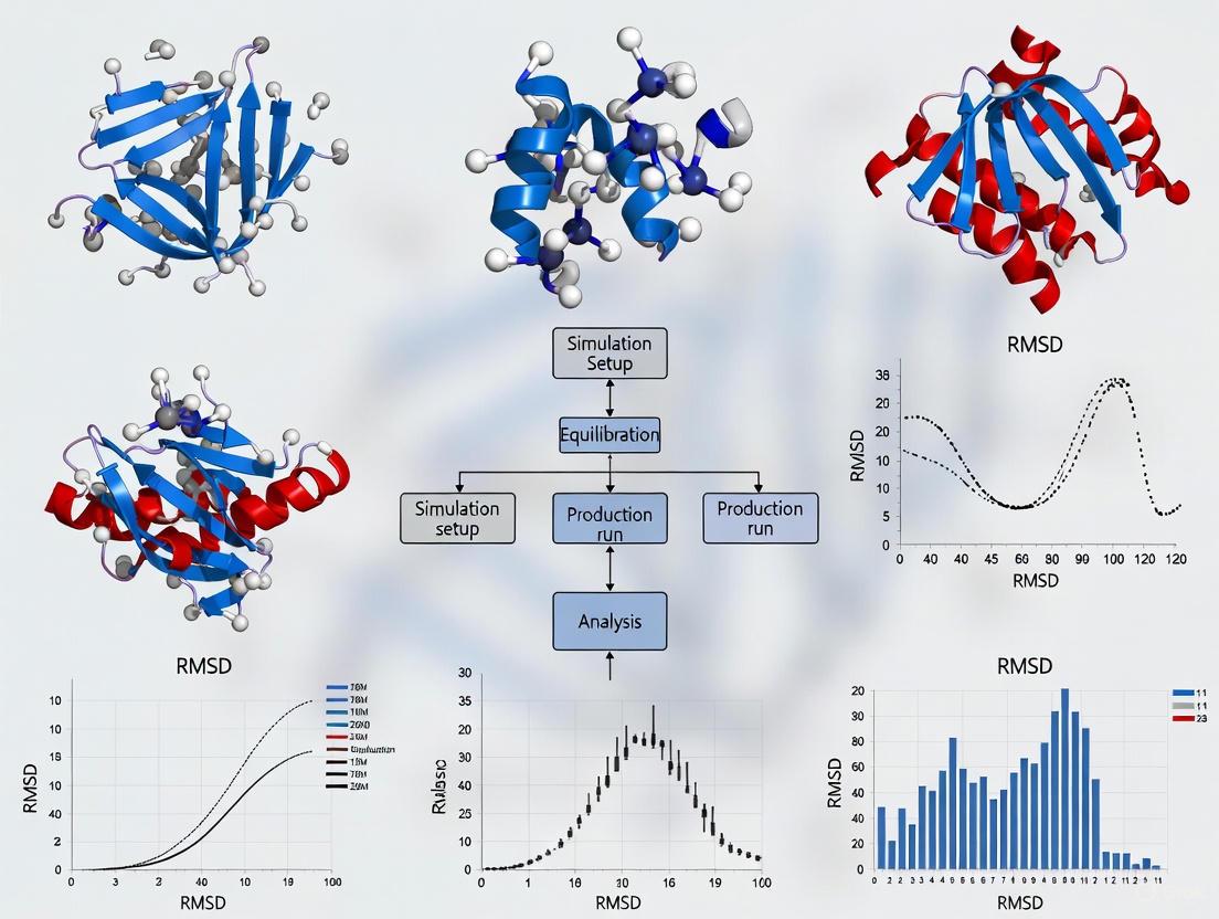
Workflow Visualization
RMSD Analysis Workflow
Advanced Applications and Guidelines
Practical Considerations for RMSD Interpretation
Effective application of RMSD analysis requires careful consideration of several factors:
- Starting Model Quality: Research indicates that MD simulations (and consequent RMSD analysis) provide the most value when applied to already high-quality starting models. For RNA structures, short simulations (10-50 ns) can modestly improve good models but rarely benefit poor models, which often deteriorate further [10].
- Simulation Length: Longer simulations (>50 ns) may induce structural drift and reduce fidelity to the experimental structure. Shorter, targeted simulations often provide more reliable refinement [10].
- Comparative Analysis: When comparing multiple structures or conformations, ensure consistent selection of reference structures, fitting atoms, and calculation parameters to enable valid comparisons.
Emerging Applications in Drug Development
Recent advances have expanded RMSD applications in pharmaceutical research:
- Machine Learning Integration: RMSD values serve as important features in machine learning models predicting drug properties such as aqueous solubility, with studies demonstrating that RMSD combined with other MD-derived properties can achieve high predictive accuracy (R² = 0.87) for solubility prediction [8].
- Ensemble Docking: RMSD-based clustering of MD trajectories helps identify representative conformations for ensemble docking, accounting for receptor flexibility in drug screening [7].
- Multi-Scale Modeling: Combined all-atom/coarse-grained approaches use RMSD to validate mixed-resolution models and ensure structural integrity while reducing computational costs for large systems [7].
Table 3: Comparison of RMSD Variants and Applications
| RMSD Type | Calculation Method | Best Suited Applications | Key Advantages |
|---|---|---|---|
| Standard Atomic RMSD | Optimal superposition of atomic coordinates | Protein folding studies, general stability assessment | Intuitive interpretation, wide software support |
| Backbone RMSD | Superposition using only backbone atoms (Cα, C, N, O) | Protein structural comparison, dynamics of globular domains | Reduced noise from flexible side chains |
| Ligand RMSD | Measurement of ligand heavy atom positions | Binding mode stability, conformational selection in drug binding | Direct assessment of ligand behavior in binding site |
| Fit-free RMSD | Based on interatomic distances without superposition | Systems where alignment is problematic, distance-based similarity | Avoids alignment artifacts, complementary perspective |
| 7x7 Matrix RMSD | Successive fitting of individual TM helices in GPCRs | Quantifying helix movements in membrane proteins | Detailed mechanistic insights into relative helix orientations |
RMSD remains an indispensable quantitative measure in structural biology and drug discovery, providing critical insights into molecular stability, conformational dynamics, and structural relationships. Its applications span from basic structural validation to advanced drug design workflows, where it integrates with multidisciplinary approaches including MD simulations, machine learning, and experimental validation. As computational methods continue to evolve, RMSD maintains its fundamental role as a robust, interpretable metric for quantifying structural deviations—a cornerstone of molecular dynamics analysis and rational drug development.
Root Mean Square Deviation (RMSD) is a foundational metric in structural biology and computational chemistry, serving as a quantitative measure of the average distance between atoms of superimposed molecular structures. The RMSD provides a single numerical value that captures the structural similarity or dissimilarity between conformational states, making it indispensable for monitoring structural changes in molecular dynamics (MD) simulations, evaluating protein structure predictions, and assessing the quality of molecular docking experiments [11] [12] [2]. For researchers and drug development professionals, understanding the mathematical formulation of RMSD is crucial for proper interpretation of results and avoidance of common pitfalls in structural analysis.
The significance of RMSD extends across numerous applications in molecular analysis. In drug discovery, RMSD calculations help validate docking poses by comparing predicted ligand conformations to experimentally determined structures [13]. In molecular dynamics simulations, RMSD tracks protein folding pathways, conformational changes, and system stability over time [8] [14]. The metric also plays a vital role in assessing structural ensembles from NMR spectroscopy, comparing crystal structures, and analyzing the effects of mutations on protein structure [12]. Despite its widespread use, the mathematical nuances of RMSD calculation and interpretation require careful consideration to ensure biologically relevant conclusions.
Mathematical Foundation of RMSD
Core RMSD Equation
The fundamental RMSD equation calculates the deviation between two sets of atomic coordinates after optimal superposition. For two structures with N equivalent atoms, the RMSD is defined as:
RMSD = √(1/N × ∑ᵢ₌₁ᴺ dᵢ²) [13]
where dᵢ represents the Euclidean distance between the coordinates of the i-th pair of corresponding atoms after optimal alignment. The calculation involves summing the squared distances between all corresponding atom pairs, dividing by the total number of atom pairs, and taking the square root of the result [11] [2]. This formulation provides a dimensioned measure (typically in Ångströms, Å) of the average structural displacement.
The mathematical derivation begins with the assumption of two coordinate sets: A = {a₁, a₂, ..., aₙ} and B = {b₁, b₂, ..., bₙ}, where each aᵢ and bᵢ represents the 3D coordinates of atoms in structures A and B, respectively. The RMSD is minimized when the structures are optimally aligned through rotation and translation, a process known as the Kabsch algorithm or Wahba's problem in more general terms [12]. The optimal alignment involves centering both structures at their centroid then finding the rotation that minimizes the sum of squared distances between corresponding points.
RMSD as an Estimator
In statistical terms, RMSD serves as an estimator for the difference between an estimated parameter and its true value. For an estimator θ̂ of parameter θ, the RMSD is defined as:
RMSD(θ̂) = √MSE(θ̂) = √E((θ̂ - θ)²) [11]
where MSE represents the Mean Square Error. For unbiased estimators, the RMSD equals the standard deviation, representing the root mean square of the differences between predicted values and observed values [11]. This statistical formulation highlights RMSD's role in quantifying predictive accuracy across various scientific domains.
Table 1: Key RMSD Equations and Their Applications
| Equation Type | Mathematical Formulation | Primary Application Context |
|---|---|---|
| Sample RMSD | RMSD = √[1/n × ∑ᵢ₌₁ⁿ(Xᵢ - x₀)²] | Comparing sample observations to true values [11] |
| Predictive RMSD | RMSD = √[∑ₜ₌₁ᵀ(yₜ - ŷₜ)²/T] | Evaluating model predictions against observed data [11] |
| Pairwise Structural RMSD | RMSD = √[∑ᵢ₌₁ᴺ ‖rᵢ - rᵢ'‖²/N] | Comparing two molecular structures after alignment [12] |
| Ensemble RMSD | <RMSD²>¹/² = √[1/Nₘ² × ∑ᵢⱼ ‖rᵢ - rⱼ‖²] | Analyzing structural diversity in molecular ensembles [12] |
Critical Considerations in RMSD Calculation
Molecular Symmetry and Atom Mapping
A significant challenge in RMSD calculation arises with symmetric molecules, where direct atomic correspondence may not reflect chemically equivalent structures. Naïve RMSD calculations that assume direct file order atomic correspondence can artificially inflate RMSD values for symmetric molecules like benzene or ibuprofen, where multiple valid atomic mappings exist [13]. For example, rotating a symmetric molecule along its axis of symmetry should yield an RMSD of zero, but incorrect atom mapping can produce erroneously high values.
Advanced approaches like the DockRMSD algorithm address this by formulating atomic correspondence as a graph isomorphism problem [13]. The algorithm:
- Represents molecules as graphs with atoms as nodes and bonds as edges
- Identifies chemically equivalent atoms through neighborhood topology matching
- Performs an exhaustive search with dead-end elimination to find the minimal RMSD mapping
- Maintains bonding network consistency throughout the mapping process
This method ensures physically meaningful atomic correspondences that respect molecular symmetry, providing biologically relevant RMSD values rather than artificially inflated measurements [13].
Normalization and Scale Dependence
RMSD is inherently scale-dependent, making direct comparisons across different molecular systems problematic [11]. A 2Å RMSD for a small drug molecule represents substantial structural deviation, while the same value for an entire protein complex might indicate remarkable similarity. To address this limitation, normalized RMSD (NRMSD) approaches have been developed:
NRMSD = RMSD/(ymax - ymin) or NRMSD = RMSD/ȳ [11]
where ymax and ymin represent the range of observed values, and ȳ represents the mean value. Normalization enables more meaningful comparisons between datasets or models with different scales [11]. The Coefficient of Variation of RMSD (CV(RMSD)) provides another normalization approach by dividing RMSD by the mean of measured data, analogous to the coefficient of variation using standard deviation [11].
For distributions with outliers, dividing RMSD by the interquartile range (IQR) creates a normalized value less sensitive to extreme values:
RMSD_IQR = RMSD/IQR where IQR = Q₃ - Q₁ [11]
This approach improves robustness when comparing systems with different levels of structural heterogeneity or when outlier conformations disproportionately influence the standard RMSD value.
Experimental Protocols for RMSD Analysis
RMSD Calculation in Molecular Dynamics Simulations
Molecular dynamics simulations generate structural trajectories that require RMSD analysis to assess conformational stability and changes. The following protocol outlines the standard workflow for RMSD analysis using VMD software:
Trajectory Loading: Load the MD trajectory file and corresponding protein structure into VMD using the "File" menu. Ensure all trajectory frames are properly read and coordinates are intact [15].
Region Selection: Access the RMSD Trajectory Tool through "Extensions" → "Analysis" → "RMSD Trajectory Tool." Select the region of interest by entering appropriate selection commands:
- Entire protein: "protein"
- Backbone only: Check "backbone" box
- Specific residues: "resid 1 to 100" [15]
Reference Frame Specification: Set the reference frame for alignment. By default, VMD uses the first frame (frame 0), but this can be modified to any frame in the trajectory based on analysis needs [15].
RMSD Calculation: Click the "RMSD" button to perform the calculation. The tool will superpose each frame onto the reference structure using the selected atoms and compute the RMSD values across the trajectory [15].
Result Visualization and Export: View results in the data table or plot RMSD versus time. Export data for further analysis by saving in the default .dat format or other compatible formats [15].
Table 2: Research Reagent Solutions for RMSD Analysis
| Tool/Software | Primary Function | Key Features | Application Context |
|---|---|---|---|
| VMD RMSD Trajectory Tool | Trajectory RMSD analysis | Built-in VMD module, backbone/specific region selection, graphical plotting [15] | MD simulation analysis, conformational stability assessment |
| DockRMSD | Symmetry-corrected RMSD | Graph isomorphism for atom mapping, MOL2 format support, open-source [13] | Docking pose comparison, symmetric molecule evaluation |
| PyMOL | Structural visualization & RMSD | Superposition algorithms, visualization of structural alignments [2] | General structural biology, publication-quality images |
| MDAnalysis | Programmatic trajectory analysis | Python library, batch processing, integration with data science workflows [2] | High-throughput analysis, custom analysis pipelines |
| GROMACS | MD simulation & analysis | Built-in RMSD modules, trajectory analysis, production-quality simulations [8] | Biomolecular simulation, force field applications |
Workflow for Docking Pose Validation
Validating docking predictions requires comparing computed ligand poses with experimental reference structures. The following protocol ensures proper RMSD calculation for docking validation:
Structure Preparation: Prepare the predicted and reference ligand structures in MOL2 format, ensuring identical atom types and bonding information. Remove water molecules and ions unless specifically relevant to the binding mode [2] [13].
Receptor Alignment: Superimpose the protein structures from the predicted and reference complexes using conserved binding site residues or the entire protein backbone. This ensures the ligand comparison occurs in the same reference frame [13].
Symmetry Assessment: Identify symmetric elements in the ligand structure, including rotatable symmetric groups, aromatic systems, and symmetric functional groups. Tools like DockRMSD automatically detect molecular symmetry through graph isomorphism searching [13].
Atom Mapping Optimization: For symmetric molecules, determine the optimal atomic correspondence that minimizes RMSD while maintaining chemical validity. DockRMSD employs an exhaustive search with dead-end elimination to identify the minimal RMSD mapping [13].
RMSD Calculation and Interpretation: Compute the symmetry-corrected RMSD and interpret results using established thresholds:
Advanced Applications and Interpretation
Relationship to Other Structural Metrics
RMSD maintains important mathematical relationships with other structural metrics. In X-ray crystallography, the ensemble-average pairwise RMSD relates to average B-factors through the equation:
<RMSD²>¹/² ∝ <B> [12]
where <B> represents the average B-factor (Debye-Waller factor). This relationship enables estimation of global structural diversity in protein ensembles directly from experimental B-factors [12]. The connection emerges from the mathematical analogy between RMSD and the radius of gyration (Rg), where pairwise RMSD distributions mirror the pairwise distance calculations used to determine Rg [12].
For RNA structural analysis, the Deformation Index (DI) incorporates RMSD but adds base interaction fidelity:
DI = RMSD/INF [16]
where INF represents the Interaction Network Fidelity calculated using the Matthews Correlation Coefficient between base-pairing and base-stacking interactions of compared structures [16]. This hybrid metric addresses RMSD's limitation in capturing the specific base interaction patterns crucial for RNA function.
Limitations and Complementary Approaches
While RMSD provides valuable global structural comparison, it has recognized limitations. RMSD spreads errors uniformly across the entire structure, making it difficult to localize structural discrepancies [16]. The metric is sensitive to outlier regions where large deviations can disproportionately influence the final value [11]. Additionally, RMSD values depend on the number of atoms included in the calculation, with all-atom RMSD typically yielding higher values than backbone-only calculations [2].
Complementary metrics address these limitations:
- Root Mean Square Fluctuation (RMSF): Analyzes local flexibility by measuring atomic position variance around average positions [12]
- Interaction Network Fidelity (INF): Quantifies reproduction of specific base-pairing and base-stacking interactions [16]
- Deformation Profile (DP): Localizes structural differences at nucleotide resolution for RNA molecules [16]
These complementary approaches combined with RMSD provide a more comprehensive structural analysis framework, particularly for complex biomolecules with specific functional interactions.
Visualization of RMSD Analysis Workflows
RMSD Analysis Workflow: This diagram illustrates the comprehensive workflow for calculating RMSD between molecular structures, highlighting critical steps including symmetry assessment and atom mapping that ensure accurate results.
RMSD Research Applications: This diagram showcases the primary research applications of RMSD calculations in molecular analysis and the key insights derived from each application area.
Within the framework of molecular dynamics (MD) analysis, the root mean square deviation (RMSD) serves as a fundamental metric for quantifying conformational similarity and tracking the evolution of a molecular system over time [17]. The reliability of any RMSD-based analysis, however, is critically dependent on two foundational elements: the choice of the initial reference structure and the application of a proper structural alignment protocol [18]. A reference structure provides the baseline coordinate set against which all subsequent conformational changes are measured, while alignment corrects for overall rotational and translational motion that is irrelevant to internal conformational dynamics [19]. Neglecting these steps can lead to RMSD values that are dominated by whole-molecule rotation and translation rather than meaningful biological fluctuations, thereby obscuring true functional insights [17] [19]. This application note details the protocols and considerations essential for ensuring that RMSD analyses accurately reflect the internal dynamics of biological macromolecules, with a specific focus on proteins and RNA nanostructures in drug development research.
Theoretical Foundation
The RMSD Metric and its Interpretation
The Root Mean Square Deviation (RMSD) is a standard measure of the average distance between atoms in two superimposed molecular structures [1]. For two sets of coordinates, v and w, each containing n equivalent atoms, the RMSD is mathematically defined as:
[RMSD(\mathbf{v}, \mathbf{w}) = \sqrt{\frac{1}{n} \sum{i=1}^{n} \|\mathbf{v}i - \mathbf{w}_i\|^2}]
In the context of MD simulations, one set of coordinates typically comes from a reference structure (e.g., the starting frame), and the other from a simulated snapshot [19]. The summation occurs over all selected atom pairs after an optimal rigid-body rotation and translation have been applied to minimize this value [1] [19]. The result is expressed in units of length (Ångströms, Å), with a value of 0 indicating perfect atomic overlap between the two structures [11] [1].
The biological interpretation of RMSD is nuanced. While a lower RMSD generally suggests greater structural similarity to the reference, and a stable RMSD over time can indicate conformational convergence, the metric suffers from degeneracy [19]. Many different conformational states can share the same RMSD value relative to a single reference. Furthermore, the global RMSD can be dominated by the displacement of a few, potentially flexible regions (like long loops or termini), masking the stability of the structural core [18]. Consequently, a careful selection of which atoms to include in the RMSD calculation is paramount for drawing biologically relevant conclusions.
The Necessity of Alignment
MD simulations allow molecules to freely rotate and translate in space. The RMSD calculated from these raw, unaligned coordinates would be artificially inflated by this global motion, providing little information about internal conformational changes, such as hinge movements in enzymes or loop rearrangements in binding pockets [17] [19].
To isolate internal dynamics, an alignment step is performed prior to RMSD calculation. This involves superposing the structure of interest onto a reference structure by finding the optimal rotation matrix and translation vector that minimize the RMSD for a selected subset of atoms, typically the stable structural core [19]. After this superposition, the RMSD is recalculated, now reflecting only the internal conformational differences. As illustrated in the protocol below, this step is crucial for obtaining a meaningful analysis of flexibility and stability [17].
Protocols for Reference Structure Selection and Alignment
Criteria for Selecting an Optimal Reference Structure
The choice of reference structure sets the baseline for all subsequent RMSD analyses. An inappropriate reference can systematically skew results and lead to incorrect interpretations.
Table 1: Criteria for Selecting a Reference Structure
| Criterion | Description | Rationale |
|---|---|---|
| Experimental Source | Prefer high-resolution structures from X-ray crystallography (<2.0 Å) or NMR ensembles [20] [18]. | Ensures atomic-level accuracy and reliability of the initial coordinates. |
| Biological Relevance | The structure should represent a functionally relevant state (e.g., active vs. inactive conformation) [18]. | Ensures dynamics are interpreted in the correct functional context. |
| Structural Completeness | The structure should have minimal missing residues, particularly in the regions of interest (e.g., active site) [20]. | Prevents artificial fluctuations due to undefined atomic positions. |
| Computational Models | For designed molecules (e.g., RNA nanostructures), use a model that has undergone energy minimization to fix steric clashes [20]. | Provides a physically realistic and stable starting point for simulation. |
A Standard Protocol for Structural Alignment and RMSD Calculation
The following protocol, adaptable for tools like MDAnalysis [17] [19] and Amber [20], outlines the key steps for proper alignment and RMSD analysis.
Step 1: Prepare the Topology and Trajectory
- Load the initial reference structure (e.g., a PDB file) and the MD trajectory file (e.g., DCD, XTC) into your analysis universe [19].
Step 2: Select Atoms for Alignment
- Choose a stable set of atoms to define the superposition. For proteins, the backbone atoms (N, Cα, C) or just the Cα atoms are commonly used, as they filter out noise from flexible side-chain motions [19]. For RNA, the phosphate backbone atoms often serve a similar purpose [20].
- Example selection in MDAnalysis:
select='backbone'orselect='name CA'[19].
Step 3: Perform Trajectory Alignment
- Iterate through each frame of the trajectory. For each frame, calculate the optimal rotation and translation that minimizes the RMSD of the selected alignment atoms to their positions in the reference frame.
- Apply this same transformation to all atoms in the system. This ensures the entire molecule (including ligands, solvent, etc.) is correctly positioned for analysis [17].
- In MDAnalysis, this is efficiently done using the
AlignTrajfunction [17].
Step 4: Calculate RMSD for Regions of Interest
- After alignment, calculate the RMSD time series. You can calculate a global RMSD using the same selection as for alignment, or, more informatively, calculate RMSD for specific domains or residues using
groupselections[19]. - Example: For adenylate kinase, one can calculate separate RMSDs for the CORE, LID, and NMP domains to quantify hinge motion independently of the stable core [19].
The workflow for this protocol is summarized in the following diagram:
Data Presentation and Analysis
Quantitative Comparison of RMSD Metrics
Presenting RMSD data effectively requires clarity about which atoms were used for both alignment and calculation. The table below demonstrates how different selections reveal distinct aspects of molecular dynamics.
Table 2: RMSD Analysis of Adenylate Kinase (AdK) Domain Motions
| Frame | Time (ns) | Global Backbone (Å) | CORE Domain (Å) | LID Domain (Å) | NMP Domain (Å) |
|---|---|---|---|---|---|
| 0 | 1.00 | 0.00 | 0.00 | 0.00 | 0.00 |
| 50 | 50.00 | 3.50 | 1.20 | 8.10 | 7.20 |
| 100 | 100.00 | 6.82 | 3.51 | 11.39 | 10.37 |
Note: Data is illustrative, based on analysis concepts from [19]. The table reveals that while the CORE domain remains relatively stable, the LID and NMP domains undergo large conformational changes, which is the functional motion of AdK. A global RMSD alone would mask this detail.
Advanced and Alternative Measures
While standard RMSD is powerful, researchers should be aware of its limitations and the availability of advanced measures.
- Weighted RMSD (wRMSD): This method uses a Gaussian weighting function during superposition, giving higher weight to atoms that move less between two conformations. This automatically focuses the alignment on the most stable structural core, providing a clearer picture of flexibility, especially for proteins with large hinged domains [21].
- Root Mean Square Fluctuation (RMSF): Unlike RMSD, which measures deviation from a reference over time, RMSF calculates the fluctuation of each atom around its average position. It is excellent for identifying flexible and rigid regions within a structure, often visualized as a plot per residue [17].
- Contact-Based Measures: These superimposition-independent methods quantify similarity based on conserved atomic or residue contacts. They are more robust than RMSD when comparing structures with significant conformational differences or domain rearrangements [18].
The Scientist's Toolkit
A successful MD analysis project relies on a suite of specialized software and resources.
Table 3: Essential Research Reagents and Software Solutions
| Tool / Resource | Function | Application Note |
|---|---|---|
| Amber | A comprehensive MD software package with specialized force fields for proteins and nucleic acids [20]. | Widely used for simulating and analyzing biomolecules; includes tools for energy minimization and MD setup [20]. |
| GROMACS | A high-performance MD simulation package, free and open-source [22]. | Known for its speed and efficiency; commonly used for large systems and long timescales [22]. |
| MDAnalysis | A Python library for analyzing MD trajectories [17] [19]. | Provides a flexible environment for scripting custom analyses, including RMSD, RMSF, and hydrogen bonding [19]. |
| VMD | A molecular visualization program with built-in analysis tools [20]. | Used for visualizing trajectories, creating publication-quality images, and initial system setup [20]. |
| Experimental Structure Database (PDB) | The primary repository for experimentally-determined macromolecular structures [18]. | The primary source for high-quality reference structures for simulations and analysis [18]. |
| Force Field (e.g., ff14SB, ff19SB) | A parameter set defining the potential energy function for atoms in a simulation [20] [23]. | The choice of force field is critical for simulation accuracy; modern force fields have significantly improved the realism of MD [20] [23]. |
The rigorous application of protocols for reference structure selection and structural alignment is not merely a preliminary step but a foundational component of meaningful MD analysis. By carefully choosing a biologically relevant, high-resolution reference and employing a proper alignment strategy focused on stable structural elements, researchers can ensure that the resulting RMSD values accurately reflect internal conformational dynamics. This, in turn, enables reliable insights into mechanisms of drug binding, allostery, and protein flexibility. As MD simulations continue to grow in importance for drug discovery, adhering to these disciplined practices will be crucial for generating robust, interpretable, and actionable data.
Root Mean Square Deviation (RMSD) is a fundamental statistical measure used to quantify the average magnitude of difference between two sets of atomic coordinates. In structural biology and computational chemistry, RMSD provides a standardized approach for assessing conformational changes, evaluating model accuracy, and measuring structural convergence in molecular dynamics (MD) simulations [11] [1]. The RMSD value represents the square root of the average of squared distances between corresponding atoms in superimposed molecular structures, typically measured in Ångströms (Å), where 1 Å equals 10⁻¹⁰ meters [1].
The mathematical formulation for calculating RMSD between two sets of atomic coordinates v and w is expressed as:
RMSD(v,w) = √[1/n × Σ‖vᵢ - wᵢ‖²] [1]
Where:
- n = number of equivalent atoms being compared
- vᵢ and wᵢ = coordinates of the i-th atom in the two structures
- ‖vᵢ - wᵢ‖ = Euclidean distance between corresponding atoms
In molecular dynamics simulations, RMSD serves as a crucial reaction coordinate for tracking structural evolution over time, providing insights into protein folding pathways, conformational stability, and the effects of ligand binding on macromolecular structure [1]. For drug discovery professionals, understanding RMSD interpretation is essential for validating docking poses, assessing predicted model quality, and making informed decisions about compound prioritization based on structural data.
Quantitative Interpretation of RMSD Values
General Guidelines for RMSD Assessment
The interpretation of RMSD values depends on contextual factors including the molecular system, comparison methodology, and research objectives. The following table provides general guidelines for interpreting global backbone RMSD values in protein structural analysis:
Table 1: General Interpretation Guidelines for Global Protein Backbone RMSD
| RMSD Range | Structural Interpretation | Typical Applications |
|---|---|---|
| < 1.0 - 1.5 Å | Very high similarity; often within experimental error or thermal fluctuation range [18] | Comparing multiple determinations of the same structure; assessing simulation convergence |
| 1.0 - 2.0 Å | High similarity; essentially identical structures [24] | Validating high-accuracy homology models; comparing closely related homologs |
| 2.0 - 3.0 Å | Moderate similarity; structurally related with some local variations [24] | Assessing acceptable homology models; comparing structures with conservative substitutions |
| 3.0 - 4.0 Å | Low similarity; notable structural differences, but potentially shared fold [24] | Detecting distant evolutionary relationships; evaluating low-accuracy models |
| > 4.0 Å | Very low similarity; substantially different structures [24] | Identifying different protein folds; rejecting poor-quality models |
Context-Dependent RMSD Evaluation
The general guidelines in Table 1 require careful consideration of specific research contexts:
Molecular size considerations: RMSD values tend to increase with protein size due to the cumulative effect of small deviations across more atoms. A 2.0 Å RMSD might indicate excellent agreement for a large multi-domain protein (e.g., >500 residues) but only moderate agreement for a small protein domain (e.g., <100 residues) [18].
Comparison scope: Global RMSD (calculated over entire structures) provides an overall similarity measure but can be dominated by flexible regions. Local RMSD (calculated over specific regions like binding sites) often provides more functionally relevant information for drug discovery applications [18] [24].
Structural flexibility: Regions with inherent flexibility (loops, termini) often exhibit higher RMSD values than structured elements (α-helices, β-sheets). Analysis should differentiate between rigid-body movements, flexible region variations, and overall structural deviations [18].
Reference structure quality: When comparing against experimental structures, consider the resolution and quality of the reference data. RMSD values near or below the experimental resolution may not be statistically significant [18].
Experimental Protocols for RMSD Analysis
Standard Workflow for RMSD Calculation in Molecular Dynamics
The following diagram illustrates the standard protocol for RMSD calculation and interpretation in MD simulations:
Protocol Details
Step 1: Structure Preparation
- Input Structures: Obtain reference and target structures in PDB format. Reference structures are typically experimental coordinates or a stable simulation frame [1].
- System Uniformity: Ensure identical atom naming, residue numbering, and chain identifiers between compared structures. Remove non-standard residues or crystallographic additives that might interfere with alignment [25].
- Protonation States: Assign appropriate protonation states for histidine residues and other titratable groups based on physiological pH (7.4) [25].
Step 2: Structural Superposition
- Alignment Algorithm: Implement the Kabsch algorithm or quaternion-based rotation for optimal rigid-body superposition, minimizing the RMSD between equivalent atoms [1].
- Reference Frame: Align all structures to a common reference frame, typically the initial simulation structure or experimental coordinates.
- Iterative Refinement: For structures with significant local variations, consider iterative superposition methods that down-weight outliers to identify the maximal common substructure [18].
Step 3: Atom Selection
- Backbone Atoms (N, Cα, C, O): Most common selection for protein structural comparisons, providing a balance between sensitivity and robustness to side-chain conformational changes [1].
- Cα Atoms Only: Simplified representation useful for large-scale comparisons and fold recognition, particularly effective for identifying global structural similarity [24].
- Binding Site Atoms: Specific selection of residues forming active sites or ligand-binding pockets, crucial for functional analysis in drug discovery [25].
- Heavy Atoms: Comprehensive comparison including all non-hydrogen atoms, most sensitive to conformational differences but susceptible to noise from side-chain rotations.
Step 4: RMSD Calculation
- Mathematical Implementation: Apply the RMSD formula after optimal superposition. Most molecular visualization and analysis packages (VMD, PyMOL, GROMACS) include built-in RMSD calculation functions [1].
- Time Series Analysis: For MD trajectories, calculate RMSD as a function of simulation time to monitor structural stability and convergence.
- Ensemble Comparisons: When comparing structural ensembles, calculate pairwise RMSD matrices to assess overall conformational diversity.
Step 5: Interpretation and Validation
- Contextual Analysis: Interpret RMSD values relative to system-specific benchmarks (see Table 1) and research objectives.
- Complementary Metrics: Validate findings using additional structural similarity measures (TM-score, GDT, RMSF) to ensure robust conclusions [18] [24].
- Statistical Significance: Assess whether observed RMSD differences are statistically significant through replicate simulations or ensemble comparisons.
Protocol for Docking Pose Validation Using RMSD
The application of RMSD in validating molecular docking predictions requires specific methodological considerations:
Experimental Workflow
Table 2: RMSD Protocol for Docking Validation
| Step | Procedure | Critical Parameters |
|---|---|---|
| Preparation | Prepare protein and ligand structures using molecular visualization software (AutoDockTools, OpenBabel) [25]. | Gasteiger charges, protonation states at pH 7.4, removal of crystallographic water molecules [25]. |
| Reference Setup | Obtain experimental ligand-protein complex structure as reference. | High-resolution crystal structure (<2.5 Å) with minimal missing residues in binding site. |
| Docking Execution | Perform molecular docking using preferred software (AutoDock Vina, QuickVina-w) [25]. | Appropriate search space dimensions; for blind docking, box size slightly larger than protein dimensions [25]. |
| Pose Extraction | Extract top-ranked docking poses based on scoring function. | Multiple poses (typically 5-20) should be considered to account for scoring function limitations. |
| RMSD Calculation | Superimpose protein structures, then calculate ligand heavy atom RMSD between docked and crystallographic poses. | Optimal rigid-body superposition of protein binding site residues prior to ligand comparison. |
| Validation | Compare calculated RMSD against acceptance thresholds. | Poses with RMSD < 2.0 Å generally considered successful predictions [25]. |
Performance Expectations
- Site-Specific Docking: When the binding site is known and appropriately defined, success rates (RMSD < 2.0 Å) typically approach 90% for standard docking benchmarks like CASF-2016 [25].
- Blind Docking: When searching the entire protein surface, success rates decrease substantially to approximately 34-47% (RMSD < 2.0 Å) due to increased search space and false minima [25].
- Exhaustiveness Settings: Higher exhaustiveness parameters in docking software can improve accuracy but increase computational cost 8-fold or more [25].
Complementary Metrics for Structural Comparison
Limitations of RMSD and Alternative Approaches
While RMSD remains widely used, several limitations necessitate complementary assessment metrics:
- Sensitivity to Outliers: RMSD is dominated by the largest deviations in a structure, meaning that a small region with large structural differences can disproportionately influence the global RMSD value [11] [18].
- Size Dependency: Global RMSD values tend to increase with protein size, making comparisons between different-sized proteins problematic [18].
- Alignment Dependence: RMSD calculation requires prior structural alignment, and different alignment methods can produce substantially different RMSD values [18].
- Limited Functional Relevance: Global RMSD may not correlate with functional properties, as key functional regions might be conserved while other regions diverge [18].
Integrated Assessment Framework
The following diagram illustrates how multiple metrics provide complementary structural information:
Table 3: Complementary Structural Comparison Metrics
| Metric | Type | Interpretation | Advantages Over RMSD |
|---|---|---|---|
| TM-score | Global | Normalized score (0,1]; >0.5 indicates same fold; <0.17 random similarity [24] | Size-independent; better fold-level discrimination; more intuitive interpretation [24] |
| GDT (Global Distance Test) | Global | Percentage of residues under specific distance cutoffs (e.g., 1Å, 2Å, 4Å) [24] | Less sensitive to outliers; emphasizes conserved regions; standard in CASP assessments [24] |
| LDDT (Local Distance Difference Test) | Local | Score (0-100) assessing local distance differences; >80 high quality [24] | Superposition-independent; evaluates local environment preservation; used in AlphaFold2 [24] |
| RMSF (Root Mean Square Fluctuation) | Local | Measures deviation from average position over time [1] | Quantifies flexibility; identifies rigid vs. flexible regions in dynamics simulations [1] |
Application in Drug Discovery: Case Studies and Protocols
Research Reagent Solutions for RMSD Analysis
Table 4: Essential Computational Tools for RMSD Analysis
| Tool/Category | Specific Examples | Application in RMSD Analysis |
|---|---|---|
| Molecular Dynamics Software | GROMACS [8], AMBER, NAMD | Perform MD simulations and calculate RMSD time series with built-in functions |
| Trajectory Analysis Tools | MDAnalysis, MDTraj, CPPTRAJ | Process simulation trajectories; compute RMSD and related properties |
| Molecular Visualization | PyMOL, VMD, ChimeraX | Structural superposition; visual validation of RMSD calculations |
| Docking Software | AutoDock Vina [25], QuickVina-w [25] | Generate ligand poses for binding mode validation via RMSD |
| Structural Alignment | Kabsch algorithm [1], Quaternions [1] | Optimal rigid-body superposition for RMSD minimization |
| Specialized Assessment | LGA [18], TM-score [24] | Implement alternative metrics to complement RMSD analysis |
Case Study: RMSD in Binding Pose Validation
A comprehensive assessment of blind docking methods on the CASF-2016 benchmark (285 protein-ligand complexes) revealed critical insights about RMSD interpretation in drug discovery contexts [25]:
- Success Rate Analysis: Only 34-47% of blind docking predictions achieved RMSD values < 2.0 Å relative to crystallographic reference structures, compared to 90.2% success for site-specific docking [25].
- Absolute RMSD Values: The median RMSD values for blind docking predictions ranged from 2.207-3.370 Å depending on software and exhaustiveness settings [25].
- Correlation with Experimental Data: Binding affinities calculated from blind docking showed very low correlation with experimental values (R² ≈ 0.15), indicating that RMSD alone does not guarantee predictive binding energy calculations [25].
Case Study: RMSD in Molecular Dynamics for Solubility Prediction
Recent research integrating MD simulations with machine learning identified RMSD as one of seven key MD-derived properties for predicting drug solubility [8]:
- Feature Importance: In a study of 211 drugs, RMSD (along with logP, SASA, Coulombic interactions, Lennard-Jones potentials, solvation free energies, and solvation shell properties) contributed significantly to accurate solubility prediction [8].
- Predictive Performance: Gradient Boosting algorithms utilizing these MD-derived properties achieved R² = 0.87 and RMSE = 0.537 for solubility prediction, demonstrating the value of RMSD in quantitative structure-property relationship models [8].
- Protocol Implementation: MD simulations were conducted in GROMACS 5.1.1 using the GROMOS 54a7 force field, with RMSD calculated for solute conformations throughout production trajectories [8].
The interpretation of RMSD values requires careful consideration of research context, system characteristics, and methodological parameters. While general guidelines suggest RMSD values below 2.0 Å indicate high structural similarity and values above 3.0-4.0 Å reflect significant differences, these thresholds must be adapted to specific applications in molecular dynamics and drug discovery. The integration of RMSD with complementary metrics like TM-score, GDT, and LDDT provides a more robust framework for structural assessment, overcoming individual limitations of each measure. For drug development professionals, RMSD remains an essential tool for validating docking poses, assessing conformational stability in MD simulations, and building predictive models of molecular properties, though its limitations necessitate careful implementation within a comprehensive structural analysis workflow.
In the post-AlphaFold era, where the prediction of static protein structures has been revolutionized by deep learning, the focus of structural biology is increasingly shifting toward understanding protein dynamics [26]. Proteins are not static entities; they function as conformational ensembles, and their biological activity is fundamentally governed by dynamic transitions between these states [26]. Within this paradigm, Root Mean Square Deviation (RMSD) analyzed as a function of simulation time serves as a crucial metric for quantifying conformational stability and tracking structural evolution in Molecular Dynamics (MD) simulations.
RMSD measures the average distance between the atoms of a simulated structure and a reference structure after optimal alignment [27]. When plotted over time, it provides a trajectory of structural change, revealing stability, unfolding events, and transitions between conformational states. This application note details the protocols for calculating and interpreting time-dependent RMSD, providing researchers and drug development professionals with the tools to integrate dynamic structural analysis into their work.
Essential Concepts and Quantitative Foundations
The RMSD Metric: A Mathematical Definition
The RMSD quantifies the deviation between two molecular structures. For a simulation trajectory, it is typically calculated for each frame ( t ) relative to a reference frame (often the initial structure at ( t=0 )) [28] [27]. The fundamental formula is:
[ RMSD(t) = \sqrt{\frac{1}{N} \sum{i=1}^N wi \lVert \mathbf{x}i(t) - \mathbf{x}i^{\text{ref}} \rVert^2} ]
where:
- ( N ) is the number of atoms used in the calculation.
- ( \mathbf{x}_i(t) ) is the position of atom ( i ) at time ( t ).
- ( \mathbf{x}_i^{\text{ref}} ) is the position of atom ( i ) in the reference structure.
- ( w_i ) is the weight assigned to atom ( i ), often its mass or simply ( 1/N ) for an unweighted average [28].
A critical step before RMSD calculation is the superposition (or fitting) of the simulated structure onto the reference structure to remove global translation and rotation, ensuring the metric reflects internal conformational changes only [28] [27]. This is often done using a subset of atoms, such as the protein backbone.
Interpreting the RMSD vs. Time Plot
The trajectory of RMSD over time provides direct insight into system behavior:
- Rapid Convergence and Stable Plateau: A system that quickly reaches a stable, low RMSD value (e.g., below 1-2 Å for a protein backbone) suggests the simulation has equilibrated and the structure is stable, closely resembling the reference [29].
- Progressive Drift: A steady, continuous increase in RMSD can indicate that the structure is undergoing a significant conformational change or drifting away from the reference state, possibly due to an inadequate force field or the lack of a necessary stabilizing factor [10].
- Sharp Jumps or Transitions: Sudden increases in RMSD often mark discrete conformational transitions, such as domain movements or partial unfolding events [30].
- High Initial Fluctuations: Large, unstable oscillations at the beginning of a simulation can suggest the initial structure is in a high-energy state and is relaxing, or that the system has not yet equilibrated.
Table 1: Key Interpreations of RMSD vs. Time Trajectories
| RMSD Profile | Structural Implication | Common Cause / Interpretation |
|---|---|---|
| Stable, Low Plateau | Conformational stability | Native state is stable under simulation conditions. |
| Progressive Drift | Conformational shift or force field inaccuracy | Ligand dissociation, domain movement, or insufficient sampling. |
| Sharp Jumps | Discrete conformational transition | Ligand binding/unbinding, allosteric change, or partial unfolding. |
| High Initial Fluctuations | System equilibration or unstable starting structure | Relaxation from a non-equilibrium starting conformation. |
Experimental Protocols and Workflows
A Standard Protocol for RMSD Analysis in GROMACS
This protocol outlines the steps for performing a basic RMSD analysis on a protein backbone using the GROMACS MD package [31] [27].
1. Simulation Preparation:
- Obtain an initial structure (e.g., from PDB, AlphaFold prediction [31]).
- Solvate the protein in a suitable water model (e.g., TIP3P) and add ions to neutralize the system.
- Minimize the energy of the system to remove steric clashes.
- Equilibrate the system, first under an NVT ensemble (constant Number of particles, Volume, and Temperature) and then under an NPT ensemble (constant Number of particles, Pressure, and Temperature).
2. Production MD Simulation:
- Run a production simulation, typically for tens to hundreds of nanoseconds, saving trajectory frames at regular intervals (e.g., every 10-100 ps).
3. Trajectory Preprocessing (Post-Simulation):
- Make the molecule whole: If periodic boundary conditions (PBC) are used, ensure molecules are not split across the box.
- Center the system: Place the protein at the center of the box.
- Remove system jumps and rotations: Fit the trajectory to a reference structure (e.g., the initial protein backbone) to remove global motion.
4. RMSD Calculation:
- Calculate the RMSD of the protein backbone (or other atom selection) over time relative to the reference structure. When prompted, select "Backbone" for both the fitting and the RMSD calculation groups.
The resulting .xvg file can be plotted to visualize RMSD as a function of simulation time.
Advanced Protocol: Multi-Domain RMSD Analysis
For proteins with multiple domains, analyzing RMSD for the entire protein can mask distinct behaviors of individual domains. This protocol, implementable in MDAnalysis [28] or GROMACS, allows for simultaneous tracking of global and local dynamics.
1. Define Atom Groups:
- Identify the atoms for the global fit (e.g., entire protein backbone).
- Define selections for specific domains or regions of interest (e.g., CORE, LID, and NMP domains as in the adenylate kinase example [28]).
2. Execute Analysis with Group Selections:
- Using MDAnalysis, the
RMSDclass can compute the RMSD for the global fit and for multiple group selections simultaneously.
Table 2: Troubleshooting Common RMSD Analysis Issues
| Problem | Potential Cause | Solution |
|---|---|---|
| RMSD never stabilizes | System is not equilibrated; protein is unfolding or undergoing large conformational change. | Check simulation parameters (temperature, pressure). Extend equilibration. Verify starting structure quality. |
| Unphysical RMSD jumps | Periodic boundary condition (PBC) artifacts; molecule is "jumping" across the box. | Use gmx trjconv -pbc whole (or equivalent) to make molecules whole before fitting and analysis [27]. |
| High RMSD from the start | Poor reference structure (e.g., low-quality model or incorrect state). | Use a high-resolution experimental structure or a high-confidence AlphaFold model (with high pLDDT) as reference [31]. |
| Noisy RMSD signal | Trajectory is not properly fitted to remove global rotation/translation. | Ensure the fitting step (-fit rot+trans in GROMACS, superposition=True in MDAnalysis) is correctly applied [28] [27]. |
Applications in Drug Discovery and Biotherapeutics
Time-dependent RMSD analysis is a cornerstone in computational drug discovery, providing critical insights into ligand binding, stability, and mechanism of action.
Evaluating Ligand-Protein Complex Stability
In virtual screening campaigns, RMSD is used to filter and prioritize hit compounds. After docking potential inhibitors into a target's binding site, MD simulations are run on the top complexes. A stable, low RMSD for both the ligand and the binding site residues indicates a stable binding pose and a promising hit [29]. For example, a study on mTOR inhibitors used RMSD to identify compounds that remained stably bound in the active site, forming key interactions with residues like VAL-2240 and TRP-2239 [29]. In contrast, a climbing RMSD for the ligand often signifies pose inversion or dissociation.
Assessing the Impact of Mutations and Environmental Changes
RMSD analysis can reveal the structural consequences of mutations or changes in environmental conditions (e.g., pH, temperature). The iGEM team at UBC Vancouver, for instance, used MD simulations at different pH levels (4, 6, 7, 9) to analyze the stability of fusion proteins for biocement applications. They monitored both RMSD and the Radius of Gyration (Rg) to understand how pH affected structural compactness and divergence from the starting conformation [31].
The Scientist's Toolkit
Table 3: Essential Research Reagents and Software for RMSD Analysis
| Tool / Resource | Type | Primary Function in RMSD Analysis | Reference / Link |
|---|---|---|---|
| GROMACS | Software Package | High-performance MD engine; includes gmx rms for RMSD calculation. |
https://www.gromacs.org [27] [8] |
| AMBER | Software Package | MD suite with cpptraj for trajectory analysis, including RMSD. |
https://ambermd.org [10] |
| MDAnalysis | Python Library | Tool for analyzing MD trajectories; flexible RMSD analysis API. | https://www.mdanalysis.org [28] |
| AlphaFold | Web Server / Software | Generates high-accuracy predicted structures for use as reference models. | https://alphafold.ebi.ac.uk [26] [31] |
| PyMOL | Molecular Viewer | Visualizes structures and trajectories; used for structural alignment and validation. | https://pymol.org [31] |
| ATLAS Database | MD Database | Repository of pre-computed MD trajectories for reference and validation. | https://www.dsimb.inserm.fr/ATLAS [26] |
Limitations and Complementary Techniques
While RMSD is indispensable, it has limitations. As a global average, it can conceal localized fluctuations and is sensitive to the choice of reference structure and fitting procedure [30]. To build a comprehensive dynamic picture, RMSD should be used in conjunction with other metrics:
- Root Mean Square Fluctuation (RMSF): Measures per-residue fluctuation around the average position, identifying flexible and rigid regions [30] [29].
- Radius of Gyration (Rg): Quantifies the overall compactness of a structure, useful for detecting unfolding or compaction events [31].
- Trajectory Maps: A novel visualization method that plots residue backbone movements as a heatmap, revealing the location, time, and magnitude of conformational changes that may be averaged out in RMSD [30].
- Principal Component Analysis (PCA): Identifies the large-scale, collective motions that account for the most variance in the trajectory, moving beyond single-atom deviations [32].
The analysis of RMSD as a function of simulation time provides a foundational, powerful lens through which to view protein dynamics. It is a critical tool for validating simulation stability, quantifying conformational changes, and assessing ligand interactions in drug discovery. While its simplicity and interpretability make it a first step in nearly all MD analyses, its true power is unlocked when used as part of a broader, multi-faceted approach that includes residue-level fluctuations, collective motion analysis, and innovative visualization. As the field moves beyond single static structures, mastering these dynamic analysis techniques, with time-dependent RMSD at their core, is essential for unraveling the mechanistic basis of protein function and regulation.
How to Calculate and Apply RMSD: Practical Protocols in Biomolecular Simulation
Root Mean Square Deviation (RMSD) is a cornerstone analysis metric in molecular dynamics (MD) simulations, providing a quantitative measure of conformational change by calculating the average distance between atoms of a macromolecule, most commonly a protein, and a reference structure over time [33]. Within the broader context of molecular dynamics analysis, RMSD serves as a fundamental tool for assessing structural stability, identifying conformational changes, and determining the convergence of a simulation towards an equilibrium state [33]. For researchers and drug development professionals, a flat or stable RMSD profile often indicates that the protein has reached a stable conformation, whereas significant jumps or sustained shifts can signal major structural rearrangements or potential simulation artefacts [33] [34]. This guide provides a detailed, step-by-step protocol for performing robust RMSD analysis on protein trajectories using GROMACS, from initial trajectory preparation to advanced analysis and troubleshooting.
Theoretical Foundation of RMSD
The RMSD calculation quantifies the deviation between two molecular structures. For a structure with N atoms, the RMSD between a given conformation (r) and a reference structure (r^ref^) is calculated using the following equation, which involves a least-squares fitting procedure before the deviation is computed [35] [33]:
$$RMSD(t) = \sqrt{\frac{1}{N}\displaystyle\sum{i=1}^N \deltai (ri(t) - ri^{ref})^2}$$
Here, r~i~^ref^ represents the coordinates of the i-th atom in the reference structure, while r~i~(t) are the coordinates of the same atom at time t in the trajectory [33]. The variable δ~i~ is a weighting factor, which is often the mass of the atom (m~i~) for mass-weighted RMSD calculations, or simply 1 for non-mass-weighted calculations [35] [36]. GROMACS can compute RMSD using different fitting strategies (e.g., rot+trans, translation, or none) and allows the user to specify different groups of atoms for the fitting and the RMSD calculation itself, providing significant flexibility in the analysis [35] [36].
An alternative, fit-free method involves calculating the RMSD based on internal distances, which is implemented in the gmx rmsdist tool [35]:
$$RMSD(t) ~=~ \left[\frac{1}{N^2}\sum{i=1}^N \sum{j=1}^N \|{\bf r}{ij}(t)-{\bf r}{ij}(0)\|^2\right]^{\frac{1}{2}}$$
This approach compares the distance r~ij~ between all pairs of atoms i and j at time t with their distances in the reference structure, eliminating the need for prior rotational and translational fitting [35].
Computational Methodology
Essential Software and Tools
A specific set of software tools is required to perform MD simulations and analyze trajectories effectively. The table below lists the key research reagent solutions and their functions in RMSD analysis.
Table 1: Research Reagent Solutions for RMSD Analysis
| Tool Name | Type/Category | Primary Function in RMSD Analysis |
|---|---|---|
| GROMACS [33] [36] | MD Simulation Suite | Provides the gmx rms and gmx confrms utilities for calculating RMSD from trajectories. |
| VMD [37] [15] | Molecular Visualization | Enables visual inspection of trajectories and offers an integrated RMSD calculation tool. |
| PyMOL [37] | Molecular Visualization | Useful for high-quality rendering of protein structures before or after simulation. |
| Grace/Matplotlib [33] [37] | Data Plotting | Software libraries for graphing the resulting RMSD data from .xvg files. |
gmx trjconv [38] [37] |
Trajectory Processing Tool | Critical for correcting periodic boundary conditions and preparing trajectories for analysis. |
Pre-analysis: Trajectory Preparation
A crucial first step before any analysis is to process the raw trajectory to account for periodic boundary conditions (PBC), which can cause molecules to appear "broken" as they diffuse across the unit cell [38]. This is done using the gmx trjconv utility:
When prompted, select "Protein" as the group to center and "System" for output [38]. This command ensures that the protein remains whole and centered in the box throughout the trajectory, creating a corrected trajectory file (md_0_10_noPBC.xtc) that should be used for all subsequent RMSD analysis to avoid artefacts [38] [39].
Core Protocol: RMSD Calculation Usinggmx rms
The primary method for RMSD calculation in GROMACS is the gmx rms command. The following workflow outlines the complete procedure.
Figure 1: A workflow diagram for calculating RMSD using the GROMACS gmx rms module.
Step 1: Basic Command Execution
The fundamental command for RMSD calculation is:
-s: Specifies the reference structure file (typically a.tpror.grofile) [33] [38].-f: Provides the corrected trajectory file (.xtc) for analysis [33].-o: Defines the output file where RMSD time series data will be stored [33].-tu ns: An optional flag to set the time unit in the output file to nanoseconds for easier interpretation [33] [38].
Step 2: Atom Selection Strategy
Upon execution, the command will prompt you to select two atom groups interactively [33]:
- Group for least-squares fit: The set of atoms used to superimpose each frame of the trajectory onto the reference structure through rotational and translational fitting. This step minimizes the RMSD due to global motion [35].
- Group for RMSD calculation: The set of atoms for which the RMSD is actually computed after the fitting is complete.
It is a standard practice for protein simulations to use the "Backbone" atoms (group 4) for both fitting and RMSD calculation, as the backbone is a good indicator of the overall protein conformational change [33] [38]. This "backbone-to-backbone" RMSD provides a core measure of structural stability. The fitting and calculation groups do not need to be identical; for example, a protein can be fitted on the backbone atoms, but the RMSD can be computed for all protein atoms [35].
To automate the selection and avoid the interactive prompts, you can pipe the selections to the command:
Advanced Applications and Variations
Using a Different Reference Structure
While the default is to use the initial frame (t=0) as a reference, you can compute the RMSD relative to any structure, such as an experimental crystal structure (e.g., from a PDB file). This is useful for assessing deviation from a native state rather than the starting structure of the simulation [38].
Here, em.tpr is assumed to contain the coordinates from the original PDB file [38].
Analyzing Specific Subsets
To calculate the RMSD for a specific protein domain, a subset of residues, or a custom group of atoms, you must first create a custom index file using gmx make_ndx [33]. You then reference this file during the RMSD calculation:
This is particularly valuable for multi-domain proteins, where analyzing individual domains can isolate local flexibility from the overall motion of the protein [39].
RMSD Matrix Analysis
A powerful analysis involves calculating the pairwise RMSD between every frame in the trajectory, generating an RMSD matrix. This can reveal transitions between distinct conformational states, which appear as blocks along the matrix diagonal [35] [36].
The -m flag directs the output to an .xpm file, which can be visualized with gmx xpm2ps or other supporting viewers [36].
Data Interpretation and Analysis
Quantitative Interpretation Guidelines
After generating an RMSD plot, correct interpretation is crucial. The following table provides general guidelines for understanding RMSD values in the context of protein stability.
Table 2: Interpretation of RMSD Values for Protein Structures
| RMSD Value (nm) | RMSD Value (Å) | Typical Interpretation | Structural Implication |
|---|---|---|---|
| 0.05 - 0.15 nm | 0.5 - 1.5 Å | Very Low | Excellent structural stability; minimal deviation from reference. |
| 0.15 - 0.25 nm | 1.5 - 2.5 Å | Low | Good stability; typical for a well-equilibrated, folded protein. |
| 0.25 - 0.35 nm | 2.5 - 3.5 Å | Moderate | Significant flexibility, possibly from loops, tails, or domain movements. |
| > 0.35 - 0.40 nm | > 3.5 - 4.0 Å | High | Large conformational changes; may indicate domain rearrangements or partial unfolding. |
It is critical to note that these values are general guidelines. Larger proteins and those with inherent flexibility, such as multi-domain proteins connected by flexible linkers, will naturally exhibit higher RMSD values (e.g., 1.5-2.5 nm) even in the absence of unfolding, due to the accumulation of small deviations across many atoms and the relative motion of domains [39]. A deviation of 2 Å (0.2 nm) is often considered a benchmark for good structural stability [34].
Visualization and Plotting
GROMACS outputs RMSD data in .xvg format, which can be plotted using various tools. The following Python code using Matplotlib provides a customizable way to visualize your results:
This script produces a clear line plot of RMSD versus time, allowing for direct observation of equilibration, stability, and any major conformational transitions [33].
Troubleshooting and Optimization
Even with a correct workflow, several common issues can affect RMSD analysis.
High RMSD Values: If your RMSD is unusually high (e.g., > 2-3 nm), first visually inspect the trajectory in a program like VMD to check for unfolding or major artefacts [39]. For multi-domain proteins, calculate the RMSD for individual domains; if domain-specific RMSDs are low (e.g., 0.2-0.5 nm) while the global RMSD is high, the large value likely arises from the relative motion of rigid domains rather than unfolding [39]. You can also try excluding highly flexible terminal residues from the RMSD calculation, as their unfolding can disproportionately influence the result [39].
Sudden Jumps in RMSD: Discrete jumps in an otherwise stable RMSD profile are often a symptom of incomplete PBC correction. Re-running the
trjconvcommand with different options (-pbc clusterfollowed by-pbc nojump) can resolve this [37] [39]. The following sequence is a more robust post-processing protocol:Assessing Convergence and Stability: A stable or "flat" RMSD curve after an initial rise is typically interpreted as the system having reached equilibrium [33]. However, RMSD alone cannot definitively prove convergence, as it is a degenerate metric—different conformational changes can produce the same RMSD value [38]. It should therefore be used in conjunction with other analyses, such as Radius of Gyration (Rg) and Root Mean Square Fluctuation (RMSF), to build a comprehensive picture of protein dynamics [39].
Root Mean Square Deviation (RMSD) is a fundamental metric in structural biology and molecular dynamics (MD) simulations for quantifying the conformational similarity between two molecular structures. It measures the average distance between the atoms of two superimposed structures, providing critical insights into protein folding, ligand binding, and structural stability over time. Within the context of a thesis on molecular dynamics analysis, mastering RMSD calculation is essential for evaluating simulation quality, assessing structural convergence, and comparing experimental vs. computed structural data. The RMSD between two coordinate sets is mathematically defined as the square root of the average squared distance between corresponding atoms after optimal superposition, calculated as:
$$ \rho(t) = \sqrt{\frac{1}{N} \sum{i=1}^N wi \left(\mathbf{x}i(t) - \mathbf{x}i^{\text{ref}}\right)^2} $$
where $N$ is the number of atoms, $\mathbf{x}i(t)$ represents the coordinates of atom $i$ at time $t$, $\mathbf{x}i^{\text{ref}}$ denotes the reference coordinates, and $w_i$ represents optional weights for each atom [40].
Theoretical Foundations of RMSD Calculation
The RMSD calculation process involves several critical theoretical considerations that ensure meaningful comparisons between molecular structures:
Optimal Superposition: The true minimal RMSD requires prior translational and rotational alignment of the structures being compared. Without this alignment, RMSD values can be misleadingly large and not reflect actual structural similarity. The alignment is typically achieved by minimizing the RMSD through translation of centroids to the origin followed by rotational alignment using algorithms like the Quaternion Characteristic Polynomial (QCP) method [41].
Atom Matching and Ordering: Accurate RMSD calculation requires that atoms in the compared structures are correctly ordered. When atomic ordering differs between structures, algorithms such as the Hungarian method for distance minimization or inertia-aligned reordering must be employed to find optimal atom mapping [41].
Weighting Schemes: RMSD calculations can incorporate weighting factors, often based on atomic masses. These weights $wi$ are normalized relative to their mean value ($wi = \frac{w'_i}{\langle w' \rangle}$) to compute a weighted average that can emphasize the contribution of specific atoms to the overall structural deviation [40].
Essential Tools and Libraries for RMSD Analysis
The MDAnalysis library provides a comprehensive toolkit for RMSD analysis of molecular dynamics trajectories, offering implementations of sophisticated algorithms alongside user-friendly interfaces. Key advantages of this library include its compatibility with common trajectory formats (LAMMPS Dump, VASP POSCAR, XYZ, PDB), integration with the scientific Python ecosystem, and use of fast C++ accelerated code through the TaiChi project [42].
Table 1: Essential Research Reagent Solutions for RMSD Analysis
| Component | Function in RMSD Analysis | Implementation Notes |
|---|---|---|
| MDAnalysis Library | Primary Python library for handling trajectory data and performing RMSD calculations | Provides RMSD analysis class and rmsd() function; requires NumPy [40] |
| Trajectory Files | Storage of atomic coordinates across simulation frames | Common formats: LAMMPS Dump, PDB, XYZ; must be whole molecules for PBC [42] [40] |
| Reference Structure | Baseline conformation for structural comparison | Typically first frame, crystal structure, or minimized structure [40] |
| Atom Selection | Defines subset of atoms for alignment and calculation | Common: "backbone" for proteins; specified via selection strings [40] |
| QCP Algorithm | Efficient calculation of optimal rotation for superposition | Implementation in MDAnalysis.lib.qcprot; essential for minimal RMSD [40] [41] |
Protocol: Calculating RMSD Using MDAnalysis
This section provides a detailed, step-by-step protocol for performing RMSD analysis on MD trajectories using MDAnalysis, suitable for researchers investigating protein dynamics in drug discovery.
System Preparation and Trajectory Handling
Procedure:
- Load trajectory and reference structure: Initialize Universe objects for both the trajectory and reference structure. The reference can be a separate file or a specific frame from the trajectory.
Ensure molecular integrity: For simulations with periodic boundary conditions, ensure molecules are made whole before RMSD calculation to prevent artifacts from atoms being imaged across box boundaries [40].
Define atom selections: Identify relevant atom groups for alignment and analysis. Typical selections include protein backbone atoms for structural comparison.
RMSD Calculation and Analysis Workflow
Procedure:
- Initialize the RMSD analysis object: Configure the RMSD calculator with appropriate selections and parameters.
Execute the analysis: Run the RMSD calculation across all trajectory frames.
Access and visualize results: Extract results and generate publication-quality figures.
Figure 1: Workflow for RMSD calculation and analysis using MDAnalysis.
Advanced Applications: Multi-Domain Protein Analysis
A powerful application of RMSD analysis involves investigating relative domain movements in multi-domain proteins, which is particularly relevant for understanding allosteric mechanisms in drug targets. The example below demonstrates analyzing domain-specific RMSD for adenylate kinase, a protein that undergoes large conformational changes between open and closed states [40].
Procedure:
- Define domain-specific selections: Identify residue ranges corresponding to structural domains.
Perform multi-group RMSD analysis: The
groupselectionsparameter enables simultaneous calculation of RMSD for both the overall structure and specific domains after superposition based on the main selection.Interpret domain motions: Differential RMSD patterns across domains reveal conformational flexibility and structural transitions.
Table 2: Example RMSD Values for Adenylate Kinase Domains
| Time (ps) | Overall RMSD (Å) | CORE Domain RMSD (Å) | LID Domain RMSD (Å) | NMP Domain RMSD (Å) |
|---|---|---|---|---|
| 0 | 0.00 | 0.00 | 0.00 | 0.00 |
| 200 | 1.85 | 0.92 | 3.45 | 2.78 |
| 400 | 2.34 | 1.12 | 4.67 | 3.92 |
| 600 | 2.78 | 1.45 | 5.23 | 4.56 |
| 800 | 2.91 | 1.62 | 5.47 | 4.81 |
| 1000 | 3.12 | 1.73 | 5.89 | 5.12 |
Figure 2: Multi-domain RMSD analysis workflow for identifying differential domain motions.
Critical Considerations and Troubleshooting
Several technical considerations are essential for robust RMSD analysis in research settings:
Periodic Boundary Conditions: For MD simulations with periodic boundaries, ensure molecules are made whole before RMSD calculation to prevent artificial inflation of RMSD values due to atoms being split across periodic images [40].
Alignment Artifacts: Be cautious when interpreting RMSD for highly flexible systems. Large-scale domain movements can dominate the alignment, masking smaller but functionally important structural changes. In such cases, domain-specific alignment may be more informative.
Statistical Significance: When comparing RMSD values between different systems or conditions, employ statistical tests to assess significance, particularly given the time-correlated nature of MD trajectories.
Memory Management: For large trajectories, consider memory-efficient approaches such as on-the-fly RMSD calculation or chunked analysis to avoid loading entire trajectories into memory.
RMSD calculation using Python and MDAnalysis provides an indispensable toolset for molecular dynamics analysis in structural biology and drug discovery research. The protocols outlined in this application note establish a foundation for quantifying structural deviations, investigating domain motions, and validating simulation stability. When implemented following the detailed methodologies presented, RMSD analysis serves as a robust approach for characterizing conformational dynamics, with particular utility for understanding allosteric mechanisms and ligand-induced structural changes in pharmaceutical development. The integration of these computational approaches with experimental structural data enables researchers to establish meaningful correlations between molecular flexibility and biological function.
Root Mean Square Deviation (RMSD) is a fundamental metric in molecular dynamics (MD) simulations for quantifying the structural evolution and stability of biomolecular systems. It measures the average distance between atoms of superimposed structures, providing crucial insights into conformational changes over time [1]. In the context of a broader thesis on MD analysis, the protocol for selecting atoms for RMSD calculation is not merely a technical step but a critical determinant of the biological interpretation. The choice of atoms—whether the protein backbone, the entire protein, or specific ligands—directly influences the assessment of structural convergence, flexibility, and binding mode stability, which are paramount for applications in structural biology and rational drug design.
This application note details standardized protocols for RMSD analysis, emphasizing the selection of appropriate atom subsets to answer specific research questions. The procedures are designed for use with the GROMACS MD suite, a robust and widely adopted tool in the computational community [43]. We provide detailed methodologies, structured data presentation, and visual workflows to ensure researchers can reliably apply these techniques to their systems of interest, from simple proteins to complex protein-ligand complexes.
Theoretical Foundation and Quantitative Comparisons
The RMSD Equation and Its Interpretation
The RMSD is calculated as the square root of the mean squared distance between corresponding atoms after optimal superposition [44] [1]. For two sets of ( N ) equivalent atom vectors, ( \mathbf{v} ) and ( \mathbf{w} ), the RMSD is formally defined by:
[ RMSD(\mathbf{v}, \mathbf{w}) = \sqrt{\frac{1}{N}\sum{i=1}^{N} \| \mathbf{v}i - \mathbf{w}i \|^2 } = \sqrt{\frac{1}{N}\sum{i=1}^{N} \left( (v{ix}-w{ix})^2 + (v{iy}-w{iy})^2 + (v{iz}-w{iz})^2 \right) } ]
The result is expressed in length units, typically Ångströms (Å) or nanometers (nm) [1]. The most common practice for protein structural comparison is to perform a rigid-body superposition that minimizes the RMSD, and this minimum value is reported [1]. The measure can be computed for all atoms, but is most frequently applied to the backbone atoms (N, Cα, C) or sometimes exclusively to the Cα atoms [1].
Comparative Analysis of RMSD Atom Selection Strategies
The selection of atoms for RMSD fitting and calculation directly impacts the numerical value and its scientific meaning. The table below summarizes the primary strategies, their applications, and key considerations.
Table 1: Protocol Selection Guide for RMSD Analysis in MD Simulations
| Analysis Target | Recommended Fitting Group | Recommended RMSD Calculation Group | Typical Reference Structure | Key Insights Provided | Common Pitfalls |
|---|---|---|---|---|---|
| Overall Protein Fold & Stability | Protein Backbone | Protein Backbone | Initial simulation frame (t=0) or experimental structure | Global conformational stability and large-scale structural changes. | High values may indicate unfolding or domain shuffling, but can be skewed by flexible terminal loops [45]. |
| Protein Side Chain Dynamics | Protein Backbone | All Protein Heavy Atoms | Initial simulation frame (t=0) | Conformational rearrangements of side chains, relevant for allosteric sites or enzyme active sites. | Can be noisy; high values may not necessarily indicate global instability. |
| Ligand Binding Mode Stability | Protein Backbone | Ligand Heavy Atoms | First frame of the simulation | Ligand's positional and orientational stability within the binding pocket [46]. | Incorrect selection (fitting ligand on ligand) reports only internal ligand flexibility, not its movement relative to the protein [46]. |
| Internal Ligand Flexibility | Ligand Heavy Atoms | Ligand Heavy Atoms | First frame of the simulation | Conformational stability and internal dynamics of the ligand itself. | Does not provide information on the ligand's position relative to the binding site. |
Experimental Protocols for RMSD Analysis
General Workflow for MD Simulation and Analysis
The following diagram outlines the comprehensive workflow for setting up, running, and analyzing a molecular dynamics simulation, with emphasis on the RMSD analysis steps detailed in subsequent protocols.
Protocol 1: Protein Backbone RMSD for Fold Stability
Purpose: To assess the stability of the protein's overall fold and secondary structure during the simulation.
Procedure:
- Trajectory Preparation: Correct for periodic boundary conditions and center the system in the box. Using GROMACS, this is typically done with the
trjconvmodule. Select "Protein" for centering and "System" for output.
- RMSD Calculation: Calculate the backbone RMSD by performing a least-squares fit to the backbone of the reference structure (usually the starting structure).
When prompted:
- For least-squares fit: Select
Backbone. - For RMSD calculation: Select
Backbone.
- For least-squares fit: Select
Interpretation: A stable, plateaued RMSD value indicates that the protein has equilibrated and its global fold is stable. A steadily increasing RMSD may suggest unfolding or a large conformational transition. Note that high RMSD values can sometimes be caused by flexible terminal or loop regions rather than core instability, so visualization is recommended [45].
Protocol 2: Whole Protein Heavy Atom RMSD
Purpose: To evaluate conformational changes that include side chain rearrangements across the entire protein structure.
Procedure:
- Trajectory Preparation: Use the same preprocessed trajectory from Step 3.2.1 (
md_0_1_noPBC.xtc).
- RMSD Calculation: Perform the fit on the backbone to remove global rotation/translation, but calculate the RMSD for all heavy atoms.
When prompted:
- For least-squares fit: Select
Backbone. - For RMSD calculation: Select
Protein(or the group containing all non-solvent, non-ion heavy atoms).
- For least-squares fit: Select
Interpretation: This RMSD will generally be higher than the backbone-only RMSD due to the inherent flexibility of side chains. It is useful for studying systems where side chain dynamics are functionally important.
Protocol 3: Ligand-Specific RMSD for Binding Stability
Purpose: To monitor the stability of a ligand's position and orientation within its binding pocket.
Procedure:
- Trajectory Preparation (Critical): Ensure the trajectory is fitted to the protein backbone to provide a consistent frame of reference for measuring ligand movement. Select "Backbone" for the fitting group and "System" for output.
- Ligand RMSD Calculation: Calculate the RMSD of the ligand's heavy atoms relative to the protein backbone.
When prompted:
- For least-squares fit: Select
Backbone[46]. - For RMSD calculation: Select
Ligand(a custom group you may need to create).
- For least-squares fit: Select
Interpretation: A low, stable ligand RMSD (e.g., ~0.1-0.3 nm) suggests a stable binding pose. A high or fluctuating RMSD may indicate weak binding, an incorrect initial pose, or multiple binding modes. Caution: Selecting the ligand for both fitting and calculation will only report the ligand's internal flexibility, giving a deceptively low RMSD and misrepresenting its true positional stability [46].
Advanced Applications and Integration with Modern Structural Tools
RMSD Analysis in the Era of AlphaFold2
The integration of high-accuracy protein structure predictions from AlphaFold2 (AF2) with MD simulations presents new opportunities and considerations for RMSD analysis. AF2 models have demonstrated remarkable performance in docking studies, sometimes comparable to experimental structures [47]. However, systematic evaluations reveal that AF2 can show limitations in capturing the full spectrum of biologically relevant states, particularly in flexible regions and ligand-binding pockets [48]. For instance, AF2 has been shown to systematically underestimate ligand-binding pocket volumes and capture only single conformational states in systems where experimental structures show functionally important asymmetry [48].
When using an AF2 model as the starting structure for MD, the RMSD analysis protocol remains the same. However, the interpretation should be nuanced. The initial rise in RMSD may not only reflect relaxation from a crystal structure but also refinement of the predicted model towards a more physiologically realistic conformation. This is especially relevant for regions with low pLDDT confidence scores, which often indicate intrinsic disorder or regions requiring stabilisation by binding partners [48]. Comparing the MD-relaxed AF2 model to experimental structures (if available) via RMSD can provide valuable insights into the model's predictive accuracy and the dynamic behavior of the protein.
The Scientist's Toolkit: Essential Research Reagents and Software
Table 2: Essential Tools for MD Simulations and RMSD Analysis
| Tool/Reagent | Category | Function | Example/Note |
|---|---|---|---|
| GROMACS | MD Software Suite | Performs high-performance MD simulations and subsequent trajectory analysis [43]. | Includes gmx rms for RMSD calculations. |
| AMBER99SB-ILDN | Force Field | Defines potential energy functions and parameters for proteins and nucleic acids. | A widely used and well-tested force field for biomolecular simulations [49]. |
| TIP3P | Water Model | Defines the geometry and interaction parameters for water molecules in the simulation. | A standard 3-site water model [43]. |
| VMD / PyMOL | Visualization Software | Used for visual inspection of the initial structure, simulation trajectories, and specific conformational states. | Critical for validating RMSD results and identifying structural causes for RMSD changes. |
| StreaMD | Automation Tool | Python-based tool that automates the setup, execution, and analysis of MD simulations [49]. | Reduces manual errors and facilitates high-throughput simulation workflows. |
| AlphaFold DB | Structure Repository | Source for high-confidence predicted protein structures to be used as initial coordinates. | Always check the per-residue pLDDT confidence metric [48]. |
The selection of atoms for RMSD analysis is a deliberate choice that should be driven by the specific biological question. As detailed in these protocols, using the protein backbone is ideal for assessing global fold stability, while including all heavy atoms provides a view of side chain dynamics. For protein-ligand complexes, the critical practice is to fit on the protein backbone and calculate the RMSD for the ligand to accurately monitor its binding pose stability. With the advent of predictive models like AlphaFold2 and automated simulation tools, these robust RMSD analysis protocols remain a cornerstone for validating structural models, assessing simulation stability, and deriving meaningful insights into biomolecular function and drug binding.
Within the framework of molecular dynamics (MD) analysis, Root Mean Square Deviation (RMSD) serves as a fundamental metric for quantifying the stability and conformational dynamics of biomolecular systems. In structure-based drug design, validating the stability of a ligand within its target's binding pocket is crucial for confirming binding modes and assessing the potential efficacy of a drug candidate [50]. This case study examines the application of RMSD analysis to evaluate the binding stability of a natural compound, 1,3-Bis(1H-benzimidazol-2-yl)propan-1-amine (STOCK1N-05528), within the binding groove of the EZH2 receptor, a target in cancer therapeutics [51]. The study leverages a 50-nanosecond MD simulation to compare the conformational stability of the ligand in both wild-type and mutant (Y641F, A677G) EZH2 receptors, providing a practical protocol for employing RMSD in binding stability validation.
Experimental Setup and System Preparation
Protein-Ligand Complex Construction
The initial crystal structure of the EZH2 receptor (PDB) featured a partially missing binding groove in its catalytic SET domain, rendering it unsuitable for docking studies [51]. To overcome this, the researchers employed a homology modeling approach:
- Modeling Software: The SET domain binding groove was remodeled using Modeller for both the wild-type and mutant (Y641F and A677G) EZH2 receptors [51].
- Ligand Docking: The top-ranked natural compound, STOCK1N-05528, was identified via virtual screening and molecular docking using GLIDE within the Schrödinger Suite [51]. The docking protocol involved extra precision (XP) mode, yielding a glide G-score of -11.664 kcal/mol for the wild-type and -12.26 kcal/mol for the mutant complex, indicating superior binding in the mutant [51].
System Preparation for Molecular Dynamics
The modeled protein-ligand complexes were prepared for simulation to ensure a physiologically relevant environment [51]:
- Protonation States: Ionizable residues were set to their standard protonation states at physiological pH.
- Solvation: The system was solvated in an explicit water model (e.g., TIP3P) within a predefined box size.
- Neutralization: Ions (e.g., Na⁺ or Cl⁻) were added to neutralize the system's net charge.
- Energy Minimization: The entire system underwent energy minimization to remove steric clashes and bad contacts, using tools like the Protein Preparation Wizard in Maestro [52].
Table 1: Key Research Reagent Solutions and Software Tools
| Resource Name | Type/Category | Primary Function in Workflow |
|---|---|---|
| Modeller | Homology Modeling Software | Reconstruct missing or incomplete binding site regions for molecular docking [51]. |
| GLIDE (Schrödinger) | Molecular Docking Software | Predict binding poses and affinity of ligands within a prepared protein receptor [51]. |
| CHARMM/GROMACS | Molecular Dynamics Engine | Perform energy minimization, equilibration, and production MD simulations [53] [51]. |
| Maestro Protein Prep Wizard | System Preparation Tool | Add hydrogens, assign partial charges, and optimize hydrogen bonding networks [52]. |
| PyMOL/Molecular Viewer | Visualization and Analysis Software | Visually inspect trajectories, binding poses, and conformational changes [51]. |
Molecular Dynamics Simulation Protocol
Simulation Parameters
The MD simulations were conducted to capture the dynamic behavior of the protein-ligand complexes [51]:
- Software and Force Field: Simulations were performed using GROMACS or CHARMM with the CHARMM36 or similar all-atom force field to model interatomic interactions [53] [51].
- System Setup: The solvated and neutralized systems were first energy-minimized and subsequently equilibrated in two phases:
- NVT Ensemble: Equilibration of particle number, volume, and temperature (typically ~100 ps) to stabilize the system temperature.
- NPT Ensemble: Equilibration of particle number, pressure, and temperature (typically ~100 ps) to achieve the correct system density.
- Production Run: A production MD simulation was carried out for 50 nanoseconds for each system under constant temperature (e.g., 300 K) and pressure (1 atm) using the Berendsen or Parrinello-Rahman barostat [51].
- Trajectory Saving: The atomic coordinates were saved every 10-100 picoseconds for subsequent analysis.
RMSD Analysis Methodology
The stability of the protein-ligand complex was assessed by calculating the RMSD of the protein's C-alpha atoms and the heavy atoms of the ligand relative to the initial simulation frame [51]. The RMSD is calculated using the formula:
[ \text{RMSD}(t) = \sqrt{\frac{1}{N} \sum{i=1}^{N} |\vec{r}i(t) - \vec{r}_i^{\text{ref}}|^2} ]
Where:
- ( N ) is the number of atoms (C-alpha for protein, heavy atoms for ligand)
- ( \vec{r}_i(t) ) is the position of atom ( i ) at time ( t )
- ( \vec{r}_i^{\text{ref}} ) is the reference position of atom ( i ) (usually from the initial frame)
This analysis was performed on the wild-type and mutant EZH2 complexes to compare their relative stability [51].
Results and Analysis
Quantitative RMSD Stability Assessment
The RMSD analysis provided a direct measure of the structural stability and convergence of the protein-ligand complexes over the simulation time.
Table 2: RMSD and Energetic Analysis of EZH2-Ligand Complexes
| System | Final System Energy (kcal/mol) | Protein C-alpha RMSD | Ligand Heavy Atom RMSD | Equilibration Time (ns) | Key Interaction Residues |
|---|---|---|---|---|---|
| Wild-type EZH2 Complex | -84,978.25 | ~4.2 Å (after 10 ns) | Fluctuations observed | ~5 ns | Y726, F667 [51] |
| Mutant EZH2 Complex (Y641F, A677G) | -84,992.23 | ~4.3 Å (stable after 10 ns) | More stable profile | ~8 ns | F665 (interaction lost with G677) [51] |
The data reveals that the mutant complex achieved a slightly lower final energy and maintained a stable RMSD after equilibration, whereas the wild-type complex exhibited more fluctuations, suggesting the mutation impacted the conformational landscape and ligand binding stability [51].
Integration with Complementary Analyses
To gain a comprehensive understanding, RMSD data was interpreted alongside other analytical metrics:
- Root Mean Square Fluctuation (RMSF): Quantified per-residue flexibility. The wild-type system showed higher flexibility in residues 100-110 and 150 compared to the mutant, indicating mutation-induced changes in local dynamics [51].
- Residue Interaction Network (RIN) Analysis: Revealed that the A677G mutation disrupted a key hydrogen bond with residue F665, altering the local interaction network and potentially contributing to the observed RMSD stability differences [51].
- Principal Component Analysis (PCA) & Free Energy Landscape (FEL): PCA showed distinct collective motions between the wild-type and mutant systems. The mutant system's FEL indicated a lowest energy minimum of 0.5 kcal/mol compared to 0.08 kcal/mol for the wild-type, confirming the mutation affected the overall conformational stability and funnelled the system into a different low-energy state [51].
The workflow below illustrates the integrated process from system preparation to multi-faceted analysis.
This case study demonstrates that RMSD is a critical, though not standalone, metric for validating ligand binding stability. The mutant EZH2-ligand complex showed a more stable RMSD profile and lower system energy, suggesting that the mutations (Y641F, A677G) stabilized the ligand binding mode, corroborated by the improved docking score [51]. The integration of RMSD with RMSF, PCA, and FEL provided a multi-dimensional view of the system's dynamics, revealing that the mutation not only stabilized the ligand but also altered the protein's global conformational sampling and residue interaction network [51].
For researchers, this underscores a best-practice protocol: using RMSD to first identify stable binding, then applying more specialized analyses to uncover the underlying structural and energetic reasons for that stability. This approach is vital for prioritizing drug candidates in structure-based design, especially for challenging targets like the EZH2 receptor in cancer. Future work could involve longer simulation times (e.g., >100 ns) and advanced sampling methods like Binding Pose Metadynamics (BPMD) to further quantify pose stability and its correlation with experimental binding affinities [52].
Within the broader context of molecular dynamics (MD) analysis, Root Mean Square Deviation (RMSD) serves as a fundamental metric for assessing the stability of a biomolecular system by measuring its average conformational change from a reference structure over time [54]. However, a comprehensive understanding of molecular behavior requires the integration of RMSD with complementary analytical techniques. While RMSD provides a global picture of stability, Root Mean Square Fluctuation (RMSF) reveals local flexibility at the residue level, and Principal Component Analysis (PCA) reduces the complexity of the trajectory data to identify large-scale, collective motions responsible for the essential dynamics of the protein [55] [56]. Used in concert, these methods form a powerful, multi-faceted framework for interpreting MD simulations, moving beyond simple stability checks to a deeper analysis of functional mechanisms, allosteric regulation, and ligand-binding effects [55]. This protocol details the methodology for this integrated analytical approach, targeting researchers and drug development professionals.
Integrated Analysis Workflow
The following diagram outlines the core workflow for conducting an integrated MD trajectory analysis, from simulation setup to the combined interpretation of RMSD, RMSF, and PCA.
Key Analytical Metrics and Their Interpretation
The table below defines the core metrics used in this integrated analysis and guides their interpretation.
Table 1: Key Metrics for Integrated MD Trajectory Analysis
| Metric | Computational Definition | Key Interpretation | Compliments RMSD By | ||
|---|---|---|---|---|---|
| RMSD (Root Mean Square Deviation) | (\text{RMSD}(t) = \sqrt{\frac{1}{N} \sum_{i=1}^{N} | ri(t) - ri^{\text{ref}} | ^2}) Where (ri(t)) and (ri^{\text{ref}}) are the position of atom (i) at time (t) and in the reference structure, and (N) is the number of atoms [54]. | Measures global structural stability. A stable simulation plateau indicates the structure has equilibrated. | Serves as the baseline measurement for system stability. |
| RMSF (Root Mean Square Fluctuation) | (\text{RMSF}(i) = \sqrt{\frac{1}{T} \sum_{t=1}^{T} \langle | ri(t) - \langle ri \rangle | ^2 \rangle}) Where (\langle r_i \rangle) is the average position of atom (i) over the simulation time (T) [54]. | Quantifies local flexibility per residue. Peaks often indicate flexible loops, termini, or functionally important regions [29]. | Explaining which parts of the structure are responsible for the deviations seen in the global RMSD. |
| PCA (Principal Component Analysis) | Diagonalization of the covariance matrix of atomic positional fluctuations to obtain eigenvectors (principal components, PCs) and eigenvalues (variance) [55]. | Identifies large-scale collective motions. The first few PCs often describe biologically relevant conformational changes [55] [56]. | Revealing the collective motions and conformational sampling that underlie the RMSD values, providing a mechanistic view. |
Experimental Protocol: Integrated Trajectory Analysis
This section provides a detailed, step-by-step protocol for performing an integrated RMSD, RMSF, and PCA analysis on an MD trajectory using common tools like GROMACS and MDAnalysis.
Prerequisite: Trajectory Preparation
Before analysis, ensure your trajectory is properly prepared. This typically involves centering the protein in the simulation box and correcting for periodic boundary conditions (PBC) to ensure molecules are whole and continuous. This is a critical step to avoid artificial fluctuations in your analysis [57].
Step-by-Step Analytical Procedure
RMSD Calculation and Analysis
- Objective: Assess the global convergence and stability of the protein backbone or a protein-ligand complex.
- Command (GROMACS):
(Use
-tu nsto output time in nanoseconds. The-sflag provides the reference structure, often the energy-minimized or starting structure.) - Interpretation: Plot RMSD vs. Time. A trajectory that has equilibrated will show a stable plateau. Significant divergence or multiple plateaus may suggest conformational sampling of different states [29].
RMSF Calculation and Analysis
- Objective: Identify regions of high flexibility and rigidity within the protein, such as flexible loops, binding sites, or stable secondary structures.
- Command (GROMACS):
(The
-resflag outputs fluctuations per residue.) - Interpretation: Plot RMSF vs. Residue Number. Correlate peaks with known structural features. In drug discovery, low fluctuation in a binding pocket can indicate stable ligand binding [29].
Principal Component Analysis (PCA)
- Objective: Extract the large-scale, collective motions that dominate the trajectory's conformational space.
- Procedure: a. Build Covariance Matrix: Calculate the covariance matrix of atomic coordinates (typically Cα atoms) after fitting to a reference structure to remove global translation and rotation. b. Diagonalize Matrix: This step is performed internally by the software, generating eigenvectors (PCs) and eigenvalues (their amplitudes). c. Project Trajectory: Project the trajectory onto the first few principal components to visualize the sampled conformational space.
- Interpretation: A 2D projection of the first two PCs (PC1 vs. PC2) can reveal distinct conformational clusters (macrostates) that may not be apparent from RMSD analysis alone [55].
Correlation and Joint Interpretation
This is the most critical phase. Cross-reference the results from the individual analyses:
- If RMSD shows multiple plateaus, use the PCA projection to confirm if these correspond to distinct, well-separated conformational clusters [55].
- Use RMSF to identify if the collective motions described by the top PCs are driven by specific flexible regions of the protein.
- In a protein-ligand complex study, compare the RMSF and PCA results of the bound and unbound systems to quantify the ligand-induced stabilization and changes in conformational dynamics [55].
The Scientist's Toolkit: Essential Research Reagents and Software
Table 2: Key Research Reagent Solutions for Integrated MD Analysis
| Tool / Resource | Type | Primary Function in Analysis |
|---|---|---|
| GROMACS [58] [57] | MD Simulation Software | High-performance engine for running simulations and performing core analyses (RMSD, RMSF, PCA). |
| MDAnalysis [55] | Python Library | Flexible toolkit for complex trajectory analysis and custom script development in Python. |
| DynamiSpectra [59] | Python Package/Web Tool | Automates analysis of multiple simulation replicas, calculating RMSD, RMSF, PCA, and more with descriptive statistics. |
| CHAPERONg [58] | Automation Tool (Bash/Python) | Automates entire GROMACS-based simulation and analysis pipelines, ideal for high-throughput studies. |
| AMBER99SB-ILDN [29] | Force Field | Provides empirical parameters for simulating proteins and calculating interatomic forces. |
| GAFF (General AMBER Force Field) [29] [57] | Force Field | Provides parameters for small organic molecules (ligands) within a simulation. |
| Flare (Cresset) [55] | Commercial Software | Provides GUI-based tools for MD analysis, including visualization of PCA results and free energy calculations. |
Application Note: mTOR Inhibitor Screening
A study on discovering ATP-competitive inhibitors of the mTOR protein showcases the power of this integrated approach. After virtual screening, the stability of the top ligand-protein complexes was evaluated using MD simulations [29].
- RMSD Analysis: The backbone RMSD of the complexes reached a stable plateau, indicating that the simulations had equilibrated and were suitable for further analysis [29].
- RMSF Analysis: Per-residue fluctuations were calculated, confirming that the binding site residues (e.g., VAL-2240, TRP-2239) exhibited low flexibility, which is characteristic of a stable binding pocket [29].
- Integrated Interpretation: The combination of stable global RMSD and low local RMSF in the binding site provided strong evidence for the structural stability of the complexes. This data, combined with analysis of specific interactions like hydrogen bonds and hydrophobic contacts, allowed researchers to identify compounds Top1, Top2, and Top6 as the most promising candidates for further inhibitor development [29]. This case demonstrates how moving beyond a single-metric assessment leads to more reliable hit selection in drug discovery.
Beyond the Plateau: Troubleshooting Common RMSD Pitfalls and Optimization Strategies
In molecular dynamics (MD) simulations, the Root Mean Square Deviation (RMSD) is one of the most ubiquitously employed metrics for assessing structural stability and convergence. A trajectory is often considered "equilibrated" once the RMSD time series appears to stabilize, forming a visually apparent plateau. This practice, however, masks a significant convergence fallacy that can compromise the interpretation of simulation data. Relying solely on an RMSD plateau as an indicator of equilibrium is a potentially misleading oversimplification. A stabilized RMSD does not guarantee that the system has sampled a representative portion of the conformational space required to compute meaningful thermodynamic or biological properties. This article deconstructs the RMSD plateau fallacy, provides robust methodologies for true convergence assessment, and illustrates these principles with a contemporary case study from antiviral research.
The Theoretical Pitfall: Deconstructing the Plateau
The standard protocol for MD simulation analysis is predicated on the assumption that the system reaches thermodynamic equilibrium. A common, yet flawed, method to verify this is to monitor properties like potential energy or RMSD, and assume equilibrium is achieved once these values reach a "relatively constant value" or a plateau [60] [61]. This approach is fraught with theoretical and practical challenges.
Partial vs. Full Equilibrium
A critical concept often overlooked is the distinction between partial equilibrium and full thermodynamic equilibrium [60] [61]. A system can be in a state of partial equilibrium where some average properties, such as inter-domain distances, have converged because they depend predominantly on high-probability regions of the conformational space (Ω). However, properties that depend explicitly on low-probability regions, such as transition rates between conformational states or the free energy, may remain unconverged [60] [61]. The RMSD is an average property; its plateau suggests stability relative to an initial structure but does not confirm adequate sampling of the entire relevant conformational landscape.
Table 1: Key Concepts in MD Convergence Analysis
| Concept | Description | Implication for RMSD |
|---|---|---|
| Partial Equilibrium | Some average properties have stabilized, relying on high-probability conformational regions. | An RMSD plateau indicates partial equilibrium at best. |
| Full Thermodynamic Equilibrium | The system has thoroughly explored all physically accessible conformational space, including low-probability regions. | Cannot be confirmed by an RMSD plateau alone. |
| Convergence Time (tc) | The time after which the running average of a property shows only small fluctuations. | The point at which the RMSD plateau is observed is not necessarily tc for other properties. |
A Practical Definition of Convergence
A more rigorous, operational definition of convergence for an MD trajectory of length T for a property Ai is as follows: Let 〈Ai〉(t) be the average of Ai calculated from time 0 to t. The property is considered "equilibrated" if the fluctuations of 〈Ai〉(t) with respect to 〈Ai〉(T) remain small for a significant portion of the trajectory after a convergence time tc, where 0 < tc < T [60] [61]. This definition highlights that judging convergence is often "more of an art than a precise determination," as a system might be trapped in a deep local energy minimum, only to escape in a longer simulation [60] [61].
The following diagram illustrates the deceptive nature of an RMSD plateau and the path to robust convergence assessment.
Essential Protocols for Convergence Assessment
To move beyond the RMSD fallacy, researchers must adopt a multi-faceted validation strategy. The following protocol outlines a robust workflow for confirming convergence in MD simulations.
A Multi-Probe Convergence Assessment Workflow
Protocol 1: Comprehensive Convergence Analysis
Objective: To verify true equilibration and adequate conformational sampling in an MD trajectory using a suite of complementary metrics.
Procedure:
- Extended Simulation Time: Recognize that multi-microsecond trajectories are often required for biologically interesting properties to converge, although full convergence of all properties (e.g., transition rates) may demand even longer timescales [60] [61].
- Multi-Metric Monitoring:
- Root Mean Square Fluctuation (RMSF): Calculate per-residue RMSF to assess flexibility and identify rigid and flexible regions. Convergence is suggested when the RMSF profile stabilizes across independent trajectory segments.
- Radius of Gyration (Rg): Monitor the compactness of the structure. A stable Rg time series complements the RMSD data.
- Secondary Structure Analysis: Use tools like DSSP to track the stability of alpha-helices and beta-sheets over time.
- Potential Energy: Ensure the total potential energy of the system has stabilized, indicating energetic equilibrium.
- Cluster Analysis: Perform clustering (e.g., using GROMACS tools) on the conformational ensemble. A well-converged simulation will show visits to all major cluster families without discovering significant new clusters in the latter halves of the trajectory.
- Block Averaging: For a key property of interest (e.g., a binding pocket distance or solvation free energy), calculate the average in successive blocks of the trajectory. The property is likely converged when the block averages show no systematic drift and their variance is acceptably small.
- Principle Component Analysis (PCA): Perform PCA on the atomic coordinates. Project the trajectory onto the first few principal components (PCs) and plot the density of conformations. A well-sampled, equilibrated system will show a smooth, unimodal or stable multi-modal density plot. Compare the density from the first and second halves of the trajectory to check for consistency.
The workflow for this rigorous analysis is summarized below.
Case Study: Aptamer-Capsid Protein Interactions
A 2025 study on a truncated DNA aptamer (TrAptm-1) binding to Macrobrachium rosenbergii nodavirus (MrNV) capsid proteins provides a concrete example of sophisticated MD analysis that looks beyond simple RMSD plateaus [62].
Experimental Protocol
Protocol 2: Microsecond-Scale MD and Energetics Analysis [62]
System Preparation:
- Software & Force Field: Simulations performed with GROMACS using the CHARMM36 force field.
- System Building: Initial complexes from molecular docking were solvated and neutralized with counterions using CHARMM-GUI. Systems contained ~222,000 atoms (monomeric complex) and ~606,000 atoms (trimeric complex).
- Equilibration: A two-step process was employed:
- NVT Equilibration: System equilibrated at 300 K using the v-scale thermostat for 125 ps.
- NPT Equilibration: System pressure stabilized at 1 bar using the Berendsen barostat for 125 ps.
Production Simulation and Analysis:
- Production Run: A 1 µs (1000 ns) production simulation was executed under NPT conditions using a 2 fs time step.
- Stability Metrics: RMSD and Root Mean Square Fluctuation (RMSF) were calculated to analyze complex stability and regional flexibility over the entire trajectory.
- Energetic Analysis: The Molecular Mechanics Poisson-Boltzmann Surface Area (MM/PBSA) method was used to calculate binding free energies. A total of 1000 snapshots from the production trajectory were analyzed to ensure statistical robustness.
Key Findings and Relevance to Convergence
The study found that the aptamer-trimeric capsid protein complex exhibited higher RMSD values (~1.2–1.5 nm) compared to the monomeric complex (~0.5–0.8 nm), indicating larger structural rearrangements [62]. Crucially, the authors did not rely on the RMSD plateau alone. They extended simulations to the microsecond scale to capture "slow conformational rearrangements characteristic of large oligomeric protein complexes" and complemented RMSD with MM/PBSA calculations, which revealed a stronger binding affinity for the trimeric capsid protein [62]. This demonstrates a modern approach where RMSD is one component of a multi-faceted analysis, rather than the sole arbiter of convergence.
Table 2: Research Reagent Solutions for MD Convergence Studies
| Reagent / Tool | Type | Function in Analysis |
|---|---|---|
| GROMACS | Software Suite | A molecular dynamics simulation package used for performing energy minimization, equilibration, and production runs. |
| CHARMM36 Force Field | Parameter Set | Defines molecular interactions (bonded and non-bonded) for proteins, nucleic acids, and lipids during the simulation. |
| CHARMM-GUI | Web-Based Tool | Used for building complex molecular systems, generating input files, and setting up simulation parameters. |
| gmx_MMPBSA | Analysis Tool | Calculates binding free energies from MD trajectories using the MM/PBSA method, providing energetic insights. |
| V-Rescale Thermostat | Algorithm | Maintains a constant simulation temperature during NVT equilibration and production. |
| C-Rescale Barostat | Algorithm | Maintains a constant pressure during NPT production simulations. |
| Particle Mesh Ewald (PME) | Algorithm | Handles long-range electrostatic interactions accurately, which is critical for simulation stability. |
The Scientist's Toolkit: Key Reagents and Computational Tools
Based on the cited research, the following table details essential resources for conducting rigorous MD studies with robust convergence analysis.
The "plateau" in an RMSD time series is a seductive but potentially misleading indicator of convergence in molecular dynamics simulations. It may signal a state of local stability or partial equilibrium but fails to confirm adequate sampling of the conformational landscape, particularly for low-probability but biologically crucial states. Robust validation requires a multi-pronged strategy that includes monitoring a suite of structural and energetic properties, employing statistical checks like block averaging, and, where necessary, extending simulation times to the microsecond scale. By moving beyond the RMSD fallacy and adopting the comprehensive protocols outlined herein, researchers can place their MD-based insights on a much firmer thermodynamic foundation, thereby enhancing the reliability of conclusions in drug discovery and structural biology.
Root Mean Square Deviation (RMSD) is a fundamental metric in molecular dynamics (MD) simulations, quantifying the structural deviation of a molecule from a reference structure over time. While its calculation is straightforward for rigid proteins, managing RMSD analysis for highly flexible molecules, particularly RNA, presents unique computational and interpretive challenges. RNA's highly charged backbone, structural plasticity, and dependence on metal ions create a complex energy landscape where traditional RMSD analysis can be misleading [63]. Furthermore, the functional relevance of RNA often lies in its dynamic conformational ensembles, which single-reference RMSD values fail to capture adequately. This Application Note details the specific RMSD challenges encountered in simulating flexible molecules and provides validated protocols to enhance the reliability of MD-based structural analysis, supporting efforts in RNA-focused drug discovery [64].
Quantitative Challenges in RMSD Analysis for Flexible Systems
Table 1: Performance of MD Simulations in RNA Structural Refinement and Folding
| System Type | Simulation Length | Key RMSD Findings | Success Rate / Performance | Primary Challenge |
|---|---|---|---|---|
| RNA Models (CASP15) [10] | 10–50 ns | Modest improvement for high-quality starting models; deterioration for poor models. | Effective for fine-tuning reliable models only. | Structural drift and reduced fidelity in longer simulations (>50 ns). |
| RNA Stem-Loop Folding [65] | Not Specified | Stem regions: < 2 Å RMSD; Loop regions: ~4 Å RMSD. | 23 out of 26 stem-loops folded successfully. | Accurate prediction of non-canonical base pairs and loop regions. |
The data in Table 1 underscores a critical point: the success of an MD simulation is highly dependent on the quality of the initial structure. For RNA, short simulations (10-50 ns) can stabilize key interactions like base stacking in pre-folded, high-quality models [10]. However, attempting to refine poorly predicted models with MD is generally unsuccessful and often leads to structural degradation. The data also highlights that different regions of a molecule exhibit varying levels of accuracy, with flexible loops presenting a greater challenge than stable stem regions, a nuance that global RMSD can easily obscure [65].
Experimental Protocols for Robust RMSD Assessment
Protocol 1: MD Refinement of RNA Structures
This protocol is designed for the targeted refinement of reliable RNA models, based on insights from the CASP15 benchmark [10].
- Starting Model Selection: Use MD refinement selectively. Run short simulations (10 ns) to quickly test model stability. Proceed with refinement only if the starting model is of high quality, as indicated by low initial RMSD and stable secondary structure during the test run.
- System Setup:
- Software: Use the Amber MD package.
- Force Field: Employ the RNA-specific
χOL3force field. - Solvation: Solvate the RNA in a TIP3P water box with a minimum 10 Å buffer.
- Neutralization: Add
MgCl2orKClto neutralize the system and achieve a physiological ion concentration of ~150 mM.
- Simulation Execution:
- Energy Minimization: Perform 5,000 steps of steepest descent minimization.
- Equilibration: Equilibrate the system in the NVT ensemble (constant Number of particles, Volume, and Temperature) for 100 ps, gradually heating to 310 K. Follow with 1 ns of NPT equilibration (constant Number of particles, Pressure, and Temperature) to stabilize the density.
- Production Run: Run a production simulation for 10-50 ns. Avoid longer simulations (>50 ns) as they often induce structural drift and reduce model fidelity [10].
- Analysis and Validation:
- Calculate RMSD relative to the initial structure, but segment the analysis for stem vs. loop regions.
- Monitor specific structural metrics: hydrogen bonding of non-canonical base pairs and stacking interactions.
- Use the refined model only if the RMSD stabilizes and key interactions are maintained or improved.
Protocol 2: Advanced Binding Free Energy Calculations for RNA-Ligand Complexes
Accurate binding affinity prediction for flexible RNA-ligand complexes requires advanced methods that go beyond standard RMSD analysis [63].
- System Preparation:
- Force Field: Utilize the AMOEBA polarizable force field for an accurate treatment of electrostatics and polarization.
- Initial Structure: Obtain the Holo (RNA-ligand complex) structure from PDB (e.g., 3TZR).
- Enhanced Sampling Simulation:
- Software & Method: Use the
lambda-Adaptive Biasing Force (lambda-ABF)scheme, combined with thedistance-to-bound-configuration (DBC)restraint scheme to improve sampling efficiency [63]. - Collective Variables (CVs): For systems with large conformational changes, employ machine learning-based CVs to capture the relevant free energy barriers.
- Software & Method: Use the
- Free Energy Calculation:
- Perform Absolute Binding Free Energy (ABFE) calculations using the parameters and pathway defined by the
lambda-ABFsimulation.
- Perform Absolute Binding Free Energy (ABFE) calculations using the parameters and pathway defined by the
- Validation:
- Compare the calculated binding affinities with experimental data (e.g., for 2-aminobenzimidazole derivatives targeting the HCV-IRES riboswitch) [63].
Protocol 3: Generating Conformational Ensembles for Flexible Binding Sites
This protocol generates plausible conformers for ensemble docking, which is crucial for flexible proteins and RNA [7].
- Mixed-Resolution Model Setup:
- Software: Use tools compatible with the Anisotropic Network Model (ANM).
- System Definition: Describe the binding site of interest at full atomistic resolution. The remainder of the protein/RNA structure is coarse-grained to reduce computational cost.
- Conformer Generation:
- Calculate the slowest three normal modes of the structure using ANM.
- Generate multiple conformers (e.g., 36) by applying deformations along these functional motion modes.
- Ligand Docking and Simulation:
- Dock the ligand into the generated conformers.
- Run multiple, independent MD simulations (e.g., 3 replicates of 100 ns) for each docked complex.
- Apply harmonic restraints (e.g., 25-50 kcal/mol·Å²) to buffer zones between the atomistic and coarse-grained regions to prevent disintegration.
- Binding Affinity Estimation:
- Use the MM-GBSA method on MD trajectories to estimate binding free energies. The 100 ns timeframe is often sufficient for convergence in such systems [7].
The Scientist's Toolkit: Essential Research Reagents and Computational Solutions
Table 2: Key Research Reagent Solutions for RNA and Flexible System MD
| Item Name | Function / Application | Key Features / Examples |
|---|---|---|
| AMBER with χOL3 [10] | MD software and force field for RNA simulation. | Provides optimized parameters for RNA nucleotides, improving stacking and sugar pucker stability. |
| AMOEBA Force Field [63] | Polarizable force field for accurate electrostatics. | Accounts for many-body polarization effects, critical for RNA's highly charged backbone and ion interactions. |
| DESRES-RNA FF [65] | Atomistic force field for RNA folding simulations. | Demonstrated high accuracy in folding diverse RNA stem-loops from unfolded states. |
| GB-neck2 Solvent Model [65] | Implicit solvent model for accelerated sampling. | Approximates solvent effects as a continuum, drastically reducing computational cost vs. explicit water. |
| lambda-ABF & DBC [63] | Enhanced sampling and restraint scheme for ABFE. | Efficiently calculates absolute binding free energies for challenging RNA-ligand complexes. |
| Anisotropic Network Model (ANM) [7] | Coarse-grained model for generating functional conformers. | Captures low-frequency, large-scale motions to create plausible structural ensembles for docking. |
Effectively managing RMSD complexity in highly flexible molecules requires a shift from a single-metric mindset to a multi-faceted strategy. The protocols and tools outlined here provide a roadmap for researchers. Key takeaways include: the selective use of MD for refinement of already stable models; the integration of advanced, polarizable force fields for physical accuracy; and the critical importance of enhanced sampling and conformational ensembles for understanding binding and dynamics. By adopting these approaches, scientists can extract more reliable and biologically meaningful insights from their molecular simulations, ultimately accelerating the development of RNA-targeted therapeutics.
Root Mean Square Deviation (RMSD) is a fundamental metric in molecular dynamics (MD) simulations, measuring the average distance between atoms of superimposed proteins or the deviation of atomic positions from a reference structure over time [11] [66]. In the context of protein folding simulations, RMSD calculations serve as a crucial measure of conformational stability and structural convergence. However, conventional RMSD analysis often incorporates atomic noise from highly flexible regions, such as solvent-exposed side chains and terminal residues, which can obscure meaningful structural signals and complicate the interpretation of simulation data.
The moving RMSD (mRMSD) methodology represents a significant advancement for analyzing protein dynamics without requiring a static reference structure [66]. This technique calculates RMSD between structures at different time points, enabling identification of stable states and metastable regions throughout the simulation trajectory. Nevertheless, the effectiveness of both conventional RMSD and mRMSD analyses depends critically on selecting appropriate atomic subsets that maximize biologically relevant signals while minimizing structural noise.
Theoretical Foundation: Atomic Contributions to Structural Noise
Mathematical Formulation of RMSD
The RMSD between two molecular structures (typically a simulation snapshot and a reference structure) is calculated as:
RMSD = √[ (1/N) × ∑ᵢ (rᵢ - rᵢ_ref)² ]
Where:
- N = Number of atoms selected for fitting and calculation
- rᵢ = Position of atom i in the current structure
- rᵢ_ref = Position of atom i in the reference structure [11]
This calculation is sensitive to outliers, as the squared error term gives disproportionate weight to atoms with large deviations [11]. In MD simulations, these large deviations often originate from functionally irrelevant structural fluctuations rather than meaningful conformational changes.
Different atomic subsets contribute variably to RMSD fluctuations:
- Backbone atoms (C, Ca, N): Generally provide the most meaningful signal for monitoring structural integrity and large-scale conformational changes
- Side-chain atoms: Often introduce significant noise due to rotational freedom and solvent interactions, though specific side chains may be crucial for analyzing functional motions
- Terminal residues: Typically exhibit higher flexibility with limited functional relevance
- Loop regions: May show substantial natural flexibility while sometimes maintaining functional importance
The optimal atom selection strategy must balance the competing needs of noise reduction and signal preservation, tailored to the specific research question and protein system under investigation.
Quantitative Analysis of Atomic Subsets for SNR Optimization
Table 1: Signal-to-Noise Characteristics of Different Atom Selections in RMSD Analysis
| Atomic Subset | Relative SNR | Best Application Context | Noise Sources | Limitations |
|---|---|---|---|---|
| Backbone only (C, Ca, N) | High | Protein folding studies, core stability assessment | Minor peptide plane fluctuations | Misses functionally relevant side-chain rearrangements |
| Heavy atoms (all non-hydrogen) | Medium-Low | Ligand-binding studies, all-atom refinement | Side-chain rotamer changes, terminal residue mobility | Susceptible to solvent-driven fluctuations |
| Alpha carbons (Cα only) | Highest | Large proteins, long timescales, domain motions | Subtle backbone rearrangements | Limited structural resolution, misses β-sheet representation |
| Core residues (buried, non-surface) | High | Thermodynamic stability, folding nuclei identification | Limited to carefully defined core | Requires prior structural knowledge |
| Structured regions (excluding termini/loops) | Medium-High | Comparative dynamics, functional motions | Depends on loop definition accuracy | May exclude functionally important flexible regions |
Table 2: mRMSD Time Interval Optimization for Different Research Objectives
| Research Objective | Recommended Interval | Optimal Atom Selection | Key Considerations |
|---|---|---|---|
| Rapid folding events | 1-10 ns | Backbone atoms | Captures secondary structure formation |
| Side-chain networking | ≥20 ns [66] | Specific functional residues | Identifies stable hydrogen bonding patterns [66] |
| Domain motions | 50-100 ns | Cα atoms | Balances computational efficiency with biological signal |
| Metastable state detection | 10-50 ns | Combined backbone + key side chains | Identifies transient intermediates with structural precision |
Experimental Protocols for Optimal Atom Selection
Protocol 1: Systematic Atomic Subset Evaluation for RMSD Analysis
Purpose: To quantitatively identify the atomic subset that maximizes SNR for a specific protein system and research question.
Materials and Reagents:
- MD simulation trajectory data (typically .dcd, .xtc, or similar format)
- Reference structure file (.pdb, .gro, or similar)
- Molecular visualization and analysis software (VMD, PyMOL, or similar)
- RMSD calculation toolkit (MDTraj, CPPTRAJ, GROMACS tools, or similar)
Procedure:
- Trajectory Preparation: Align the entire simulation trajectory to a reference structure using a consistent fitting method (typically backbone atoms)
- Atomic Subset Definition: Create multiple atomic selections representing different structural components:
- Backbone atoms (C, Ca, N, O)
- Alpha carbons only
- Heavy atoms excluding terminal residues
- Core residues (solvent accessibility < 25%)
- Structured regions (excluding residues with B-factor > mean + 1σ in crystal structure)
- RMSD Calculation: Compute RMSD time series for each atomic subset using the same reference structure
- Noise Quantification: Calculate the standard deviation of RMSD fluctuations for each subset during equilibrium phases
- Signal Identification: Identify biologically relevant conformational changes through independent methods (cluster analysis, dimensionality reduction, or experimental validation)
- SNR Optimization: Select the atomic subset that shows the clearest discrimination between functionally distinct states with minimal high-frequency fluctuations
Expected Outcomes: Identification of an atomic subset that provides at least 30-50% improvement in SNR compared to all-heavy-atom calculations, as evidenced by clearer state discrimination in RMSD distributions.
Protocol 2: Moving RMSD Analysis Without Reference Structure
Purpose: To analyze protein dynamics and identify stable states using mRMSD, eliminating potential bias from reference structure selection.
Materials and Reagents:
- MD simulation trajectory data
- Molecular dynamics analysis software with custom scripting capability (Python/MDTraj, MATLAB, or similar)
- Sufficient sampling across relevant timescales (typically ≥20 ns intervals for proper dynamics characterization) [66]
Procedure:
- Interval Selection: Choose appropriate time intervals (Δt) for mRMSD calculation based on research objectives (see Table 2)
- Atomic Selection: Apply optimal atom subsets identified through Protocol 1
- Pairwise Calculation: For each time point t, calculate RMSD between structures at time t and t+Δt across the trajectory: mRMSD(t) = RMSD(structure(t), structure(t+Δt))
- Time Series Analysis: Analyze the mRMSD trajectory to identify stable states (periods with low mRMSD) and transition states (peaks in mRMSD)
- State Validation: Extract representative structures from stable states and characterize their structural features
- Comparative Analysis: Contrast mRMSD results with conventional RMSD analysis to identify potential reference structure biases
Expected Outcomes: Identification of metastable states and characteristic structural features independent of reference structure bias, with clear discrimination between stable and transition states in the mRMSD time series.
Visualization Framework for Atom Selection Strategies
Atom Selection Optimization Workflow
Selection Strategy by Research Goal
Table 3: Essential Resources for RMSD Analysis with Optimal Atom Selection
| Resource Category | Specific Tools/Software | Primary Function | Key Features for Atom Selection |
|---|---|---|---|
| Trajectory Analysis | CPPTRAJ (AmberTools) [66] | MD trajectory analysis | Extensive atom masking capabilities, RMSD with sophisticated fitting |
| Trajectory Analysis | MDTraj (Python) | Lightweight trajectory analysis | Efficient atom selection syntax, integration with data science stack |
| Trajectory Analysis | GROMACS tools | Built-in trajectory analysis | Fast RMSD calculation, versatile index groups for atom selection |
| Visualization | VMD [66] | Trajectory visualization and analysis | Graphical atom selection, intuitive representation of atomic subsets |
| Visualization | PyMOL | Molecular visualization | High-quality rendering, structural analysis of selected subsets |
| Specialized Analysis | mRMSD scripts [66] | Reference-free dynamics | Custom implementation for pairwise RMSD calculations without reference |
| Specialized Analysis | Time series analysis (Python/R) | Statistical characterization | Noise quantification, state discrimination analysis |
| Computing Resources | Anton Supercomputer [66] | Specialized MD simulations | Ultra-long timescales for robust dynamics characterization |
| Computing Resources | GPU clusters (NAMD, OpenMM) [66] | Accelerated MD simulations | Rapid sampling for statistical significance in RMSD analysis |
In molecular dynamics (MD) and structural biology, quantifying the similarity and differences between molecular structures is fundamental. Two primary metrics for this task are the Root Mean Square Deviation (RMSD) and the Root Mean Square Deviation of Distances (RMSDist). The global RMSD is the most commonly used measure for comparing three-dimensional structures, typically calculated after an optimal rigid body superposition of one structure onto another [1] [18]. In contrast, gmx rmsdist computes the root mean square deviation of atom distances, which offers the distinct advantage that no structural fit is needed prior to calculation [67].
The choice between these metrics is not trivial and has significant implications for the interpretation of MD simulations and structural comparisons. This application note provides a detailed comparative analysis, guiding researchers and drug development professionals on the selection and application of RMSD and RMSDist based on their specific scientific objectives.
Theoretical Foundations and Definitions
Root Mean Square Deviation (RMSD)
RMSD measures the average distance between atoms (usually backbone or Cα atoms) of two superimposed molecular structures [1]. The standard calculation involves:
- Optimal Superposition: A rigid-body rotation and translation is applied to one structure (the target) to minimize its deviation from a reference structure.
- Averaging Distances: The root mean square of the distances between matched atoms is computed after superposition.
The RMSD for two sets of n equivalent atoms, after optimal superposition, is given by:
[ RMSD(\mathbf{v}, \mathbf{w}) = \sqrt{\frac{1}{n} \sum{i=1}^{n} \|vi - wi\|^2} = \sqrt{\frac{1}{n} \sum{i=1}^{n} ((v{ix}-w{ix})^2 + (v{iy}-w{iy})^2 + (v{iz}-w{iz})^2)} ]
where (vi) and (wi) are the coordinates of the (i)-th atom in the two structures [1]. The result is expressed in length units (typically Ångströms, Å), with a value of zero indicating identical structures.
RMSD of Distances (RMSDist)
RMSDist is a fit-free metric that computes the RMSD of the distances between atom pairs within a structure, comparing these internal distances to a reference [67].
The RMSDist at time t is calculated as the RMS of the differences in distance between all considered atom-pairs in the reference structure and the structure at time t. Its key feature is that it is calculated from the internal distance matrix of the structure, bypassing the need for rotational and translational fitting. This makes it inherently independent of the frame of reference.
The table below synthesizes the core characteristics of RMSD and RMSDist to guide metric selection.
Table 1: Comparative summary of RMSD and RMSDist
| Feature | Root Mean Square Deviation (RMSD) | RMSD of Distances (RMSDist) |
|---|---|---|
| Core Definition | Deviation of atomic positions after superposition [1] | Deviation of internal distances between atom pairs [67] |
| Requires Superposition? | Yes, optimal rigid-body fit is mandatory [18] | No, it is a fit-free metric [67] |
| Sensitivity to Domain Movements | Highly sensitive; large domain shifts dominate and inflate the value [18] | Robust; measures internal deformations, less dominated by large rigid shifts |
| Information Captured | Global structural similarity relative to a reference pose | Internal structural compactness and topology preservation |
| Primary Application Context | Standard measure for assessing structural convergence in MD, similarity in protein structure prediction (e.g., CASP) [1] [18] | Analyzing systems where a global fit is problematic (e.g., multi-domain proteins, intrinsically disordered regions) [67] |
| Output in GROMACS | gmx rms: Time series of RMSD [68] |
gmx rmsdist: Time series, matrices of RMSD, scaled distances, and mean distances [67] |
| Limitations | Can be dominated by a few large deviations, making it less representative of overall similarity [18] | Does not provide a direct spatial alignment, making it harder to visualize the source of differences |
When to Use Each Metric: An Application-Oriented Guide
Guidelines for Metric Selection
The following decision diagram provides a straightforward workflow for choosing between RMSD and RMSDist based on the scientific question and system characteristics.
Detailed Application Scenarios
Scenario 1: Analyzing a Single Domain Protein or Stable Complex
For a well-folded, single-domain protein or a stable protein-ligand complex, RMSD is the standard and recommended metric. The system behaves largely as a rigid body, and the primary question is its stability and fluctuations relative to the starting crystal structure.
- Protocol for RMSD Calculation using GROMACS:
- Preparation: Ensure your trajectory (
traj.xtc) and reference structure (topol.tpr) are available. Create an index file (index.ndx) containing the group of atoms to analyze (e.g.,C-alphafor backbone). - Command:
- Selection Prompts: When prompted, select the group for least-squares fitting (e.g.,
C-alpha) and then the group for RMSD calculation (e.g.,C-alpha). Using the same group ensures the structure is fitted to and evaluated on the same atoms. - Output: The
rmsd.xvgfile contains a time series of the RMSD, which can be plotted to assess equilibration and stability [68].
- Preparation: Ensure your trajectory (
Scenario 2: Analyzing Multi-Domain Proteins or Large-Scale Conformational Changes
Proteins with multiple domains often undergo hinge-like motions. In such cases, RMSDist is highly advantageous because it is not skewed by the large displacements of entire domains, focusing instead on changes within the domains themselves.
- Protocol for RMSDist Calculation using GROMACS:
- Preparation: Have your trajectory (
traj.xtc) and reference structure (topol.tpr) ready. - Command:
- Output: The
-oflag produces a time series of the average RMSDist. The-rmsflag generates an XPM matrix file showing the RMSDist between every pair of atoms over time, which is useful for identifying specific regions of flexibility [67].
- Preparation: Have your trajectory (
Scenario 3: Validating Equilibrium and Convergence
Relying solely on RMSD time series to judge simulation convergence has been criticized as subjective and potentially misleading [69]. A more robust approach is to use RMSDist in tandem with RMSD.
- Combined Protocol:
- Calculate the RMSD time series as in Scenario 1.
- Calculate the RMSDist time series as in Scenario 2.
- Comparative Analysis: A system truly at equilibrium should show stable fluctuations in both metrics. If RMSD is stable but RMSDist shows a continuous drift, it may indicate internal relaxation not apparent from the global fit, suggesting the simulation requires more time to equilibrate fully.
Experimental Protocols
Protocol 1: Standard RMSD Analysis for Stability Assessment
This protocol assesses the stability of a protein's fold during an MD simulation.
- Objective: To quantify the global structural drift of a protein backbone relative to the simulation start.
- Workflow:
- Materials - Research Reagent Solutions:
- GROMACS Suite: Open-source MD software package used for all calculations [67] [68].
- Protein Structure File: A reference structure, typically in
.tpror.groformat. - MD Trajectory File: The structural time series to be analyzed, typically in
.xtcor.trrformat. - Index File (Optional): A
.ndxfile specifying the group of atoms (e.g.,C-alpha) for analysis.
Protocol 2: RMSDist for Internal Dynamics and Topology
This protocol evaluates changes in the internal distance map, useful for analyzing flexible systems.
- Objective: To monitor internal structural changes and compactness without superposition bias.
- Workflow:
- Advanced Analysis - NOE-like Lists:
gmx rmsdistcan generate lists of atom pairs with averaged distances below a threshold (-max), useful for generating NMR-like restraint data [67]. The-equivoption allows averaging over equivalent atoms (e.g., methyl hydrogens) for direct comparison with experimental data.
RMSD and RMSDist are complementary metrics, each illuminating different aspects of structural dynamics. RMSD is the intuitive choice for assessing global stability and similarity when a meaningful superposition can be defined. RMSDist is a powerful, fit-free alternative that provides a robust measure of internal changes, especially valuable for multi-domain proteins, flexible systems, and for validating convergence without superposition bias. The informed researcher should select the metric aligned with their specific scientific question, and in many cases, employing both provides the most comprehensive insight into molecular behavior.
Root Mean Square Deviation (RMSD) is a fundamental metric in molecular dynamics (MD) simulations, quantifying the average distance in atomic positions between the structures in a simulation trajectory and a reference structure, typically the starting crystal conformation [1]. It serves as a essential measure for assessing the stability of a molecular system, identifying equilibrium phases, and confirming the convergence of a simulation [70] [71]. Despite the conceptual simplicity of RMSD, deriving scientifically sound interpretations requires a rigorous approach that accounts for statistical uncertainty, sampling quality, and potential pitfalls inherent to the simulation process [72]. This application note provides detailed protocols and best practices to ensure the robustness of your RMSD analysis within the broader context of molecular dynamics research, with a focus on applications in drug development.
Key Concepts and Statistical Foundations
A precise understanding of the terminology and statistical principles underlying uncertainty quantification is a prerequisite for robust RMSD analysis [72].
- RMSD Equation: For two molecular structures represented as sets of atomic coordinates v and w, the RMSD is calculated as shown in Table 1 [1].
- Statistical Definitions: When analyzing a time-dependent RMSD value from an MD trajectory, it should be treated as a random quantity. The arithmetic mean of RMSD values over a simulation segment provides an estimate of the expected deviation during that period. The experimental standard deviation describes the fluctuation of the RMSD around its mean, while the experimental standard deviation of the mean (often called the standard error) quantifies the uncertainty in the estimated mean RMSD value itself [72].
- Correlation Time: MD trajectories produce highly correlated data points. The correlation time (τ) is the longest separation in time between two configurations that still show significant correlation. Ignoring this correlation leads to a significant underestimation of statistical uncertainties [72].
Table 1: Key Statistical Terms for RMSD and Uncertainty Quantification
| Term | Mathematical Formula | Description and Significance in RMSD Analysis |
|---|---|---|
| Root Mean Square Deviation (RMSD) | RMSD(v,w) = √[ (1/n) * Σ‖vᵢ - wᵢ‖² ] |
Core metric for measuring structural similarity or deviation from a reference structure over time [1]. |
| Arithmetic Mean (Sample Mean) | x̄ = (1/n) * Σxⱼ |
The average RMSD value over a defined segment of the trajectory, estimating the "typical" deviation in that window [72]. |
| Experimental Standard Deviation (s(x)) | s(x) = √[ Σ(xⱼ - x̄)² / (n-1) ] |
Measures the magnitude of fluctuations of the RMSD around its mean. A stable system near equilibrium should exhibit a stable standard deviation [72]. |
| Experimental Standard Deviation of the Mean | s(x̄) = s(x) / √n |
The "standard error." Quantifies the uncertainty in the estimated mean RMSD. Critical for reporting the precision of your average stability measure [72]. |
Workflow for Robust RMSD Analysis
A systematic, tiered approach to analyzing RMSD data prevents over-interpretation and ensures conclusions are supported by sufficient evidence [72]. The following workflow outlines this process.
Pre-analysis Configuration and Checks
Before calculating RMSD, several configuration choices must be made to ensure the analysis is meaningful and reproducible.
- Atomic Selection: The choice of atoms for the RMSD calculation fundamentally influences the result. For analyzing protein backbone stability, use Cα atoms. For assessing the stability of a protein-ligand complex, calculate RMSD for the ligand's heavy atoms after superposing the protein backbone to isolate ligand movement from global protein reorientation [71].
- Structural Alignment: A rigid-body superposition that minimizes the RMSD must be performed before each calculation. This step removes global translation and rotation, isolating internal conformational changes [1]. Standard algorithms like Kabsch or quaternion-based methods are used for this purpose [1].
- Data Quality Inspection: Visually inspect the raw RMSD time series for obvious drifts, large jumps, or sudden transitions that may indicate a lack of equilibrium, the presence of rare events, or potential simulation artifacts [70].
Protocol 1: Lagged RMSD Analysis for Convergence Assessment
A critical challenge in MD is determining if a simulation has run long enough to be representative. The "lagged RMSD-analysis" method provides a robust check for non-convergence [70].
Principle: This method computes the average RMSD between all pairs of configurations in the trajectory separated by a specific time lag, Δt. By examining how this average value changes with increasing Δt, one can assess whether the simulation has sampled a stable, stationary distribution of conformations [70].
Detailed Methodology:
- Data Extraction: From an MD trajectory with
nsaved configurations, calculate ann x nmatrix of RMSD values, where each elementRMSD(i, j)is the deviation between configurations at timest_iandt_j. Most modern MD analysis packages (e.g., GROMACS'sg_rms) can perform this calculation [70]. - Compute Lagged Average: For a given time lag
Δt = k * Δt_config, calculate the average RMSD for all pairs of configurations separated by exactlyksteps:RMSD̄(Δt) = ⟨RMSD(t_i, t_i + Δt)⟩averaged over all validi[70]. - Model Fitting: Fit the resulting
RMSD̄(Δt)data to a saturation model, such as the Hill equation:RMSD̄(Δt) = (a * Δt^γ) / (τ^γ + Δt^γ), where:ais the plateau RMSD value, representing the average deviation between "independent" configurations.τis the lag time at which half-saturation occurs, related to the system's correlation time.γis the Hill coefficient governing the sigmoidicity of the curve [70].
- Interpretation: A simulation can be considered converged for a specific property when the
RMSD̄(Δt)curve has reached a stable plateau. If the curve is still increasing significantly at the maximum time lag (typically chosen as half the total simulation time), the simulation has not fully sampled the conformational space, and conclusions about stability may be premature [70].
Protocol 2: Validation Against Experimental Data
Agreement with experimental data increases confidence that the simulation force field and protocol are producing realistic conformational ensembles, not just a stable-looking RMSD profile [73].
Principle: Compare simulation-derived properties that are related to RMSD, such as Root Mean Square Fluctuation (RMSF) or NMR-derived order parameters, with experimental observations. Note that multiple conformational ensembles can yield averages consistent with experiment, so this is a necessary but not sufficient check for absolute accuracy [73].
Detailed Methodology:
- Select Comparable Observables: Calculate per-residue RMSF from the simulation, which measures the flexibility of individual residues. This can be qualitatively compared to B-factors (Debye-Waller factors) from X-ray crystallography or NMR relaxation data [73].
- Perform Multiple Replicas: Given the stochastic nature of MD, run multiple independent simulation replicas (starting from different random velocity seeds) [73]. This allows you to estimate the variance in your RMSD and RMSF results, providing an internal measure of sampling reliability.
- Quantitative Comparison: While direct RMSD comparison to experiment is often not possible, the simulated conformational ensemble should be cross-validated against any available experimental data. For instance, if a simulation predicts a large-scale conformational change, evidence from mutagenesis, spectroscopy, or other biophysical techniques should be sought to corroborate it [73].
The Scientist's Toolkit: Essential Research Reagents and Software
Table 2: Key Research Reagent Solutions for RMSD Analysis
| Item | Function in RMSD Analysis |
|---|---|
| MD Simulation Software (e.g., GROMACS, AMBER, NAMD, OpenMM) [73] [74] | Generates the raw trajectory data. The choice of software, force field, and water model can influence the resulting conformational ensemble and RMSD profile [73]. |
| Automation & Resilience Tools (e.g., drMD, custom Python scripts) [75] [74] | Manages complex simulation projects, automates restarts after interruptions, and ensures reproducibility, which is foundational for obtaining reliable, long trajectories needed for convergence [75] [74]. |
| Trajectory Analysis Suites (e.g., MDTraj, VMD, GROMACS analysis tools) [74] | Provides core functions for calculating RMSD, performing structural alignments, and conducting lagged RMSD analysis. MDTraj is a modern, open library for efficient trajectory analysis [74]. |
| Visualization Software (e.g., VMD, PyMOL) | Allows for visual inspection of trajectories and structures corresponding to specific RMSD values or transitions, providing crucial context for numerical data [74]. |
| Statistical Environments (e.g., Python with NumPy/SciPy, MATLAB, R) | Enables custom data analysis, such as fitting the Hill equation to lagged RMSD data and calculating advanced statistical measures of uncertainty [70]. |
Data Presentation and Reporting Standards
Effectively communicating RMSD results and their uncertainty is as important as the analysis itself.
Table 3: Quantitative Guidelines for Interpreting RMSD Values
| RMSD Context | Typical Value Range | Interpretation Guidance |
|---|---|---|
| Protein Backbone Stability (Cα atoms) | 1 - 3 Å | A stable, well-equilibrated globular protein often has a backbone RMSD of 1-3 Å. Values persistently above this may indicate significant conformational flexibility or lack of equilibrium [71]. |
| Protein-Ligand Complex Stability | < 2 - 3 Å | A ligand RMSD (after protein alignment) below 2-3 Å is often considered stable. Larger fluctuations may suggest weak binding or insufficient sampling [71]. |
| Re-docked Ligand Pose | < 2.0 Å | A common threshold for successful molecular docking, indicating the computational model can reproduce the crystallographically observed pose [71]. |
| Convergence Saturation (Lagged RMSD) | N/A | Convergence is indicated not by a specific value, but by the RMSD̄(Δt) curve reaching a clear plateau. The plateau value a is system-dependent [70]. |
Visualizing Data and Workflows
All figures must be clearly labeled and cited in the text. For RMSD time series plots, include a descriptive title, label axes with units (Time (ns), RMSD (Å)), and use distinct colors for different replicas or system components. When reporting mean RMSD values, always include error bars representing the standard error of the mean [72] [76] [77].
Structured Reporting in Publications
When documenting RMSD analysis in a scientific report or publication, ensure the following elements are clearly stated:
- Calculation Details: Specify the atoms used for superposition and RMSD calculation.
- Statistical Evidence: Report the mean RMSD along with its standard error or confidence interval, not just the raw value [72].
- Convergence Information: State the total simulation time and the number of independent replicas. If available, include a plot of the lagged RMSD analysis to support claims of convergence [70].
- Software and Reproducibility: Document the software and version used for both simulation and analysis to ensure reproducibility [75].
Validating Simulations and Comparing Systems: RMSD in Action for Drug Discovery
Within the framework of molecular dynamics (MD) research, the Root Mean Square Deviation (RMSD) serves as a fundamental metric for quantifying the average distance between the atoms of superimposed molecular structures, typically measured in Ångströms (Å) [1]. For researchers and drug development professionals, RMSD provides an essential, quantitative measure to validate the stability and convergence of MD simulations, which is critical for drawing reliable biological conclusions, particularly in projects investigating protein-ligand interactions, protein folding, and conformational changes [70] [78]. The core equation for RMSD calculates the deviation between two sets of atomic coordinates, often after optimal rigid body superposition to minimize the value:
$$\text{RMSD}(\mathbf{v}, \mathbf{w}) = \sqrt{\frac{1}{n}\sum{i=1}^{n}\|\mathbf{v}i - \mathbf{w}_i\|^2}$$
where $\mathbf{v}$ and $\mathbf{w}$ represent the coordinate vectors of the two structures being compared, and $n$ is the number of atoms [1]. This application note details standardized protocols for employing RMSD to benchmark both the equilibration phase and the production phase of MD simulations, ensuring the reliability of subsequent analyses.
Theoretic Foundation and Key Concepts
The RMSD Metric in Molecular Dynamics
In MD simulations, RMSD is most informatively calculated for the protein backbone or Cα atoms, as this minimizes noise from fluctuating side chains and reflects meaningful conformational shifts [79]. The analysis can be performed in two primary modes:
- Time-based RMSD: The simulation's initial frame (or a known reference crystal structure) is used as a static reference. The RMSD of each subsequent frame relative to this reference is computed, generating a time-series plot that visualizes the system's trajectory and stability over time [70] [79].
- Lagged RMSD-Analysis: This method involves calculating the RMSD between all pairs of configurations within a trajectory that are separated by a specific time lag, Δt. The average value, $\overline{\text{RMSD}}(\Delta t)$, is then plotted against Δt. The resulting curve's shape is a powerful indicator of simulation convergence; a stationary, plateaued shape suggests adequate sampling, whereas a non-stationary shape indicates the simulation may not have run long enough to escape its initial conformational basin [70].
Interpreting RMSD Profiles for Simulation Quality
The temporal evolution of RMSD provides direct insight into the simulation's stage:
- Equilibration Phase: Characterized by a sharp, often increasing RMSD trend as the system moves away from the potentially non-representative starting coordinates and relaxes into a more stable, native conformation.
- Production Phase: Marked by stable RMSD values that fluctuate around a steady average, indicating the system is sampling a stable conformational basin. The transition from the equilibration to the production phase is the point where the RMSD time-series stabilizes [70] [78].
Table 1: Summary of RMSD Types and Their Primary Applications in MD Simulation Quality Control
| RMSD Type | Definition | Primary Application in Quality Control | Key Interpretation |
|---|---|---|---|
| Time-based RMSD | RMSD of each frame relative to a single reference structure (e.g., the first frame). | Assessing overall system stability and identifying equilibration. | A stable plateau indicates convergence in a conformational basin. |
| Lagged RMSD | Average RMSD between all configuration pairs separated by a time lag Δt. | Judging the sufficiency of simulation length and conformational sampling. | A stationary $\overline{\text{RMSD}}(\Delta t)$ vs. Δt curve suggests converged sampling. |
| Blocked RMSD | RMSD averaged within sequential blocks of time. | Reducing short-term fluctuations to better reveal long-term trends. | Helps distinguish true drift from random fluctuation. |
| Weighted RMSD | RMSD calculation where atoms are weighted, e.g., by mass. | Emphasizing the contribution of specific atoms, like the protein backbone. | Provides a more relevant measure of large-scale conformational change. |
Experimental Protocols and Workflows
Comprehensive Workflow for RMSD-Based Validation
The following diagram outlines the end-to-end protocol for using RMSD to validate MD simulation quality, from system preparation to final analysis of production trajectories.
Protocol 1: Validating Equilibration with Time-Based RMSD
This protocol determines when a system has completed equilibration and is ready for production simulation.
- System Preparation: Begin with a solvated and neutralized system that has undergone energy minimization.
- Equilibration Simulation: Run a short simulation under the desired NVT (constant Number, Volume, Temperature) and/or NPT (constant Number, Pressure, Temperature) ensembles.
- Trajectory Processing: Ensure the trajectory is "whole" by correcting for periodic boundary condition effects that can fragment molecules.
RMSD Calculation:
- Software: Use packages like GROMACS (
g_rms), MDAnalysis (RMSDclass), or AMBER (cpptraj). - Selection: Typically, the protein backbone or Cα atoms are selected for the calculation.
- Reference: Use the first frame of the equilibration run (or the energy-minimized structure) as the reference.
- Command: The following example uses MDAnalysis to calculate RMSD for a trajectory against its first frame.
- Software: Use packages like GROMACS (
Visualization and Analysis: Plot the RMSD time series. The equilibration phase is complete when the RMSD value stops its initial increasing or decreasing trend and begins to fluctuate around a stable average. The simulation should be extended until this plateau is clearly observed.
Protocol 2: Assessing Production Run Quality with Lagged RMSD-Analysis
This advanced protocol judges whether a production run has been long enough to achieve converged sampling.
- Prerequisite: A production MD trajectory of sufficient length (e.g., 200 ns or more).
- RMSD Matrix Calculation: Compute an $n \times n$ matrix of RMSD values, where
nis the number of frames, containing the RMSD between every pair of framesiandj. This can be computationally demanding but is essential. - Lagged RMSD Calculation: For a range of time lags (Δt), compute the average RMSD, $\overline{\text{RMSD}}(\Delta t)$, from all pairs of frames separated by that specific lag. The maximum Δt should be no more than half the total simulation time.
Model Fitting: Fit the $\overline{\text{RMSD}}(\Delta t)$ vs. Δt data to a saturation model, such as the Hill equation, to quantify the convergence behavior:
$$\overline{\text{RMSD}}(\Delta t) = \frac{a \cdot \Delta t^\gamma}{\tau + \Delta t^\gamma}$$
Here, parameter
arepresents the plateau RMSD value,τis the lag at half-saturation, andγis the Hill coefficient [70].- Interpretation: A $\overline{\text{RMSD}}(\Delta t)$ curve that rises and then reaches a clear plateau indicates that configurations separated by lags longer than the plateau onset are statistically uncorrelated, a sign of good conformational sampling. A curve that has not yet plateaued suggests the simulation requires more time.
Case Study: RMSD in Antiviral Drug Discovery
A 2024 study on influenza PB2 inhibitors exemplifies RMSD application. After 500 ns MD simulations of protein-ligand complexes, the researchers calculated RMSD time series for both the protein backbone and the ligands. Compounds identified as promising inhibitors demonstrated low and stable RMSD values after an initial equilibration period (~50-100 ns), indicating stable binding modes and a well-equilibrated system. This stability, correlated with favorable binding free energies, was key to validating the simulations for further analysis [78].
Table 2: Exemplary RMSD Analysis from a 500 ns Simulation of a Protein-Ligand Complex [78]
| Simulation Component | Equilibration Phase Duration (approx.) | Average Production RMSD (Å) | Interpretation & Significance |
|---|---|---|---|
| Protein Backbone (Cα) | 50-100 ns | ~1.5 - 2.5 Å | The system reached a stable, folded conformation; the simulation is converged for analysis. |
| Stable Ligand (e.g., Compound 4) | 50-100 ns | ~0.5 - 1.5 Å | The ligand maintained a stable binding pose, suggesting high binding affinity. |
| Less Stable Ligand | >100 ns | >2.5 Å | The ligand's binding mode was dynamic or unstable, suggesting lower affinity. |
The Scientist's Toolkit
Table 3: Essential Software and Tools for RMSD Analysis in MD Simulations
| Tool Name | Type/Brief Description | Primary Function in RMSD Analysis |
|---|---|---|
| GROMACS | MD Simulation Suite | Includes g_rms for efficient RMSD calculation from trajectories and can generate RMSD matrices for lagged analysis [70]. |
| MDAnalysis | Python Library for MD Analysis | Provides the RMSD class for flexible RMSD calculations, allowing superposition on one atom group and calculation on another [80] [79]. |
| AMBER | MD Simulation and Analysis Suite | The cpptraj module offers powerful commands for RMSD time-series calculation and extensive trajectory analysis [78]. |
| drMD | Automated MD Pipeline | Simplifies running MD simulations for non-experts, generating trajectories that can be passed to other tools for RMSD analysis [75]. |
| OpenMM | High-Performance MD Toolkit | The engine used by drMD and others to generate simulation data; analysis typically performed with other tools [81]. |
RMSD is an indispensable, robust metric for benchmarking the quality of molecular dynamics simulations. By applying the outlined protocols—using time-based RMSD to definitively identify the equilibration plateau and employing lagged RMSD-analysis to critically assess the conformational sampling of production runs—researchers can ensure their simulations are thermodynamically stable and statistically meaningful. This rigorous validation is foundational for obtaining reliable results in computational drug discovery and molecular biology, transforming MD from a black box into a verifiable tool for scientific discovery.
In the field of structure-based drug design (SBDD), the accurate prediction of how a small molecule (ligand) binds to its protein target is a fundamental challenge. Molecular docking simulations aim to predict this binding mode, or "pose," but a critical step lies in validating these computational predictions against experimental reality. Cross-docking validation is a rigorous computational technique designed to assess the robustness of docking protocols and scoring functions by simulating a more realistic drug discovery scenario. This approach involves docking multiple ligands from a set of related protein-ligand complexes into the binding sites of non-cognate protein structures, rather than just back into their original (cognate) structures [82]. This method tests a model's ability to generalize, moving beyond simple redocking exercises to better mimic real-world applications where the protein structure may not perfectly match the ligand being docked [83]. The core metric for quantifying the accuracy of a predicted pose is the Root-Mean-Square Deviation (RMSD), which measures the average distance between the atoms of the docked pose and the experimentally determined reference pose after optimal superposition [1]. A lower RMSD value indicates a closer match to the experimental structure, with values typically below 2.0 Å considered near-native [82]. This application note details the protocols for performing cross-docking validation, framed within the broader context of molecular dynamics and RMSD analysis research.
Core Concepts and Key Metrics
The Central Role of RMSD
The Root-Mean-Square Deviation (RMSD) is the standard measure for quantifying the spatial difference between two molecular structures, such as a docked pose and an experimental crystal structure [1]. It is calculated using the formula:
RMSD = √[ (1/N) × Σ(δ_i)² ]
Where:
- N is the number of atoms being compared
- δ_i is the distance between atom i in the predicted structure and its equivalent in the reference structure after optimal rigid body superposition [1] [44].
In the study of globular proteins, the similarity of three-dimensional structures is customarily measured by the RMSD of the Cα atomic coordinates after optimal rigid body superposition [84]. For ligand pose prediction, the heavy-atom RMSD between the docking pose and the crystal pose is the standard metric, with poses possessing an RMSD of less than 2.0 Å generally classified as "near-native" [82]. While RMSD is a crucial metric, it is important to note its limitations. Relying solely on intuitive inspection of RMSD plots to determine system equilibrium in molecular dynamics simulations has been shown to be unreliable and subject to bias [69].
Cross-Docking vs. Redocking
It is critical to distinguish between redocking and cross-docking, as they assess different aspects of a scoring function's capability:
- Redocking: The process of docking a ligand back into the exact same protein structure from which it was originally crystallized. This tests a scoring function's ability to identify the correct pose under ideal, cognate conditions.
- Cross-Docking: The process of docking a ligand into a protein structure that was crystallized with a different ligand. This tests the scoring function's generalization capability and its robustness to subtle variations in binding site architecture, making it a more realistic and challenging benchmark for real-world drug discovery applications [82].
Computational Methodology and Datasets
Preparation of Cross-Docking Datasets
The foundation of a reliable cross-docking study is a carefully curated dataset. Standardized datasets are essential for fair comparison between different scoring functions and machine learning models.
- PDBbind Database: A widely used resource that provides a consolidated repository of biomolecular complexes with experimentally measured binding affinity data [82].
- CrossDocked2020: A more recent and extensive dataset specifically designed for structure-based machine learning. It contains 22.5 million poses of ligands docked into multiple similar binding pockets across the Protein Data Bank, providing a vast resource for training and benchmarking [83].
A typical protocol for dataset construction from PDBbind involves:
- Selecting the refined set from PDBbind.
- Grouping protein structures by sequence similarity to create clusters for cross-docking.
- For each cluster, docking every ligand against every non-cognate protein structure within the cluster to generate cross-docked poses [82].
Machine Learning for Pose Selection
Traditional scoring functions often struggle with the docking pose selection task. Recently, machine learning (ML) and deep learning (DL) approaches have emerged as powerful alternatives. These models are trained to either predict the RMSD value of a pose or directly classify poses as "near-native" or "decoy" based on features extracted from the protein-ligand complex [85] [82].
Common feature sets used for training these ML models include:
- Extended Connectivity Interaction Features (ECIF): Describe protein-ligand atomic interactions.
- Classical Scoring Function Energy Terms: Such as those from AutoDock Vina.
- Docking Pose Ranks: The initial ranking provided by the docking program.
- 3D Grid-based Representations: The complex is represented as a 3D grid of atom densities, which is then processed by a Convolutional Neural Network (CNN) [83] [85].
Table 1: Common Feature Sets for Machine Learning-Based Pose Prediction
| Feature Category | Description | Example Use Case |
|---|---|---|
| Interaction Features (ECIF) | Statistical potentials derived from known protein-ligand complexes. | XGBoost classifiers for pose selection [82]. |
| Energy Terms | Empirical energy components from classical scoring functions. | Augmenting ML models to improve generalization [82]. |
| 3D Grids | 3D "pictures" of the complex using atom type densities. | Input for Convolutional Neural Networks (CNNs) [83]. |
| Graph Representations | Atoms as nodes, bonds/interactions as edges. | Input for Graph Neural Networks (GNNs) [85]. |
Experimental Protocols
Protocol 1: Standard Cross-Docking Validation Pipeline
This protocol outlines the key steps for performing a cross-docking validation study using classical or machine-learning scoring functions.
Step 1: Dataset Curation and Preparation
- Obtain a curated dataset such as the CrossDocked2020 set or create one from the PDBbind refined set [83] [82].
- For a custom dataset, cluster protein targets based on sequence or structural similarity (e.g., ≥70% sequence identity) to define cross-docking groups.
- Prepare protein and ligand files, ensuring proper addition of hydrogen atoms, assignment of protonation states, and optimization of hydrogen bonding networks.
Step 2: Pose Generation via Molecular Docking
- Select a docking program (e.g., Surflex-Dock, AutoDock Vina, GNINA) to generate ligand conformations within the binding site [82].
- For each ligand, perform docking against all non-cognate protein structures within its cluster. Generate a sufficient number of poses per complex (e.g., 20-50) to ensure adequate sampling of the conformational space.
- Include the experimental (crystal) pose in the generated pose set for reference.
Step 3: Pose Scoring and Evaluation
- Calculate the heavy-atom RMSD between each generated pose and the experimental crystal structure pose using a tool like OpenBabel's
obrmsutility [82]. - Classify any pose with an RMSD below 2.0 Å as a "near-native" hit.
- For each cross-docked complex, record the RMSD of the top-scoring pose and determine if it is a success (RMSD < 2.0 Å). The overall success rate across all complexes is the primary metric for docking power assessment.
Step 4: Data Splitting for Machine Learning Models
- If evaluating ML models, avoid random splits which can lead to overoptimistic performance estimates due to data leakage between training and test sets.
- Use clustered cross-validation, where entire protein clusters are held out as the test set, ensuring that proteins in the test set are not highly similar to those in the training set. This provides a more realistic measure of a model's ability to generalize to new targets [83] [82].
Protocol 2: Assessing a Scoring Function's Docking Power
This protocol provides a standardized framework for benchmarking the pose prediction capabilities of any scoring function.
Table 2: Key Metrics for Evaluating Docking Power
| Metric | Calculation Method | Interpretation |
|---|---|---|
| Top-1 Success Rate | Percentage of complexes where the pose ranked #1 by the scoring function has an RMSD < 2.0 Å. | The primary metric for assessing a scorer's ability to identify the single best pose. |
| Success Rate within Top-N | Percentage of complexes where at least one pose in the top N ranked poses has an RMSD < 2.0 Å (e.g., N=1, 2, 3, 5, 10). | Measures the scorer's usefulness when multiple poses are considered for further analysis. |
| AUC-ROC for Pose Classification | Area Under the Receiver Operating Characteristic curve for the binary classification of poses as near-native (RMSD<2Å) or decoy (RMSD>2Å). | Evaluates the overall ranking quality across all poses, not just the top ranks. |
Procedure:
- For a set of cross-docked complexes, generate a diverse set of decoy poses for each.
- Score all poses (near-native and decoys) using the target scoring function.
- Rank the poses for each complex based on their scores.
- For each complex, calculate the RMSD of the top-ranked pose and the minimum RMSD among the top-N poses.
- Aggregate the results across all complexes to compute the metrics listed in Table 2.
Workflow Visualization
The Scientist's Toolkit: Research Reagent Solutions
Table 3: Essential Computational Tools for Cross-Docking Studies
| Tool / Resource | Type | Primary Function in Cross-Docking |
|---|---|---|
| PDBbind (http://www.pdbbind.org.cn/) | Database | Core database of protein-ligand complexes with experimental binding affinities for dataset construction [82]. |
| CrossDocked2020 | Dataset | Large-scale, standardized dataset of cross-docked poses for training and benchmarking ML models [83]. |
| AutoDock Vina / Smina | Docking Program | Widely used open-source docking software for generating ligand poses [82]. |
| GNINA | Docking Program / ML Scorer | Docking software that utilizes an ensemble of convolutional neural networks as its scoring function [83] [85]. |
| Surflex-Dock | Docking Program | Commercial docking program known for high performance in pose reproduction [82]. |
| Open Babel | Cheminformatics Tool | Used for file format conversion and RMSD calculation between poses [82]. |
| GROMACS | MD Simulation Suite | Includes tools for calculating RMSD and other analysis metrics from molecular dynamics trajectories [44] [86]. |
| Bio3D (R Package) | Analysis Tool | Provides utilities for analyzing MD trajectories and crystal structures, including RMSD, RMSF, and PCA [86]. |
Cross-docking validation has emerged as an indispensable methodology for rigorously assessing the performance of docking protocols and scoring functions in structure-based drug design. By moving beyond the artificial scenario of redocking and explicitly testing a model's ability to identify correct ligand poses in non-cognate protein structures, it provides a more realistic and meaningful benchmark for practical drug discovery applications. The integration of machine learning, particularly deep learning models trained on large-scale cross-docked datasets like CrossDocked2020, represents a significant advance in the field. These models show enhanced "docking power" and improved generalization to novel targets. As the field progresses, the continued development of standardized cross-docking datasets and robust validation protocols, grounded in rigorous RMSD analysis, will be crucial for driving the development of more reliable computational tools for predicting protein-ligand interactions.
Osteoarthritis (OA) is a prevalent degenerative joint disease and a leading cause of global disability, characterized by the irreversible degradation of articular cartilage [87]. The pathophysiology of OA involves multiple joint tissues, with matrix metalloproteinase-13 (MMP-13) playing a particularly crucial role as the primary enzyme responsible for cleaving type II collagen, the main structural component of cartilage [88] [89]. Despite the significant disease burden, current OA treatments primarily manage symptoms rather than addressing the underlying disease mechanisms, creating an urgent need for disease-modifying therapies [89].
Artesunate (ART), a natural product derivative primarily known for its antimalarial properties, has recently demonstrated potential in osteoarthritis treatment due to its anti-inflammatory and cartilage-protective capabilities [87]. Experimental studies have shown that artesunate significantly reduces the protein levels of MMP-3 and MMP-13 while suppressing inflammatory factors in chondrocytes [87]. However, the precise molecular mechanism underlying artesunate's interaction with MMP-13 remained unclear until recently.
This case study employs computational structural biology techniques—specifically molecular docking and molecular dynamics (MD) simulations—to investigate the binding behavior and stability of artesunate to MMP-13. Through root mean square deviation (RMSD) analysis, we demonstrate how artesunate achieves stable binding within the MMP-13 active site, providing mechanistic insights at the atomic level that support its potential as a novel OA therapeutic agent targeting MMP-13.
Background and Significance
MMP-13 as a Therapeutic Target in Osteoarthritis
Matrix metalloproteinases constitute a family of zinc-dependent endopeptidases that play critical roles in extracellular matrix (ECM) remodeling [88]. Among more than 25 identified MMP types, MMP-13 (collagenase-3) exhibits exceptional efficiency in degrading type II collagen, the principal collagenous component of articular cartilage [89]. The destructive capacity of MMP-13 extends beyond collagen cleavage to include induction of chondrocyte apoptosis, thereby exacerbating cartilage damage [87].
MMP-13's three-dimensional structure typically consists of three α-helices and five β-folds, with its catalytic domain containing two zinc ions: one structural and one catalytic [88]. The S1' specificity pocket and its surrounding Ω-loop have emerged as critical regions for developing selective MMP-13 inhibitors that avoid the musculoskeletal syndrome (MSS) side effects associated with early-generation, non-selective MMP inhibitors [89].
Artesunate: From Antimalarial to Potential OA Therapeutic
Artesunate is a clinically versatile artemisinin derivative with established pharmacokinetic profiles and favorable safety data from decades of antimalarial use [90]. Following administration, artesunate rapidly converts to its active metabolite, dihydroartemisinin (DHA), through esterase-catalyzed hydrolysis [90]. Intravenous artesunate demonstrates particularly rapid pharmacokinetics, with an elimination half-life of less than 15 minutes, while DHA exhibits a slightly longer half-life of 30-60 minutes [90].
Beyond its antiparasitic effects, emerging research has revealed artesunate's pleiotropic biological activities, including modulation of inflammation and apoptosis in various cell types [87]. In the context of osteoarthritis, experimental studies have demonstrated that artesunate ameliorates cartilage damage by reducing MMP-3 and MMP-13 expression while increasing type II collagen production [87]. These findings positioned artesunate as a promising candidate for OA treatment, though its direct molecular interactions with MMP-13 remained uncharacterized.
Computational Methodology
Molecular Docking Protocol
Molecular docking simulations predicted the binding orientation and affinity of artesunate within the MMP-13 active site. The protocol included these critical steps:
Protein Preparation:
- Retrieved the crystal structure of MMP-13 (PBD ID: 3OXH) from the Protein Data Bank
- Removed bound water molecules and co-crystallized ligands
- Added hydrogen atoms and assigned appropriate protonation states to ionizable residues
- Performed energy minimization using the AMBER force field to relieve steric clashes
Ligand Preparation:
- Obtained the three-dimensional structure of artesunate from PubChem database
- Optimized geometry using density functional theory at the B3LYP/6-31G* level
- Assigned Gasteiger charges and rotatable bonds for flexible docking
Docking Procedure:
- Defined the active site around the catalytic zinc ion with a 15Å grid box
- Utilized AutoDock Vina with an exhaustiveness setting of 32
- Generated 20 binding poses clustered by root mean square deviation (RMSD) tolerance of 2.0Å
- Selected the pose with the most favorable binding energy for subsequent MD simulation
Molecular Dynamics Simulation Protocol
Molecular dynamics simulations assessed the stability and dynamic behavior of the artesunate-MMP-13 complex:
System Setup:
- Solvated the protein-ligand complex in a TIP3P water box with 10Å buffer
- Added sodium and chloride ions to neutralize the system and achieve 0.15M physiological salt concentration
- Employed the AMBER ff14SB force field for the protein and GAFF parameters for artesunate
- Applied the SHAKE algorithm to constrain bonds involving hydrogen atoms
Equilibration and Production:
- Conducted energy minimization using steepest descent followed by conjugate gradient algorithms
- Performed gradual heating from 0 to 310K over 200ps in the NVT ensemble
- Equilibrated density over 500ps in the NPT ensemble at 1atm pressure
- Ran production simulation for 50ns with a 2fs integration time step
- Saved coordinates every 10ps for subsequent trajectory analysis
Trajectory Analysis:
- Calculated root mean square deviation (RMSD) to assess structural stability
- Computed root mean square fluctuation (RMSF) to identify flexible regions
- Determined binding free energy using the MM-PBSA method
- Analyzed hydrogen bonding occupancy and interaction fingerprints
Table 1: Key Parameters for Molecular Dynamics Simulation
| Parameter Category | Specific Setting | Rationale |
|---|---|---|
| Force Field | AMBER ff14SB for protein, GAFF for ligand | Accurate parameterization of biological systems |
| Water Model | TIP3P | Computational efficiency while maintaining accuracy |
| Simulation Time | 50ns production run | Sufficient for observing ligand-binding stability |
| Temperature Control | 310K using Langevin thermostat | Maintain physiological relevance |
| Pressure Control | 1atm using Berendsen barostat | Isotropic pressure coupling for biological systems |
| Electrostatics | Particle Mesh Ewald (PME) | Accurate treatment of long-range interactions |
| Constraint Algorithm | SHAKE | Allows 2fs time step by constraining bond vibrations |
RMSD Analysis Fundamentals
The root mean square deviation (RMSD) serves as a fundamental metric for quantifying structural similarity and conformational changes during molecular dynamics simulations. The RMSD between two molecular structures is calculated as:
[ \text{RMSD} = \sqrt{\frac{1}{N} \sum{i=1}^{N} \deltai^2} ]
Where (\delta_i) represents the distance between atom (i) in the reference and target structures after optimal superposition, and (N) is the number of atoms considered [28]. For protein-ligand complexes, the RMSD trajectory provides crucial insights into binding stability, with values below 2-3Å typically indicating stable binding [87].
In this study, we calculated both protein backbone RMSD (to assess overall conformational stability) and ligand heavy atom RMSD (to evaluate binding pose stability). The MDAnalysis library implementation of the fast QCP algorithm was employed for efficient RMSD computation throughout the trajectory [79].
Results and Analysis
Molecular Docking Reveals Favorable Binding Mode
Molecular docking simulations demonstrated that artesunate exhibits strong binding affinity for MMP-13, with a calculated binding energy of ≤ -7.0 kcal/mol [87]. The docking pose revealed critical interactions between artesunate and the MMP-13 active site:
Zinc Ion Coordination:
- The artesunate endoperoxide bridge positioned within coordination distance of the catalytic zinc ion
- This interaction likely contributes significantly to binding energy
Hydrogen Bonding Network:
- Artesunate formed hydrogen bonds with key residues in the S1' pocket
- The carboxylate group of artesunate interacted with polar residues in the active site
Hydrophobic Interactions:
- The nonpolar regions of artesunate established van der Waals contacts with hydrophobic residues lining the specificity pocket
- These interactions enhanced binding specificity and complementarity
Table 2: Key Interactions Between Artesunate and MMP-13 Active Site Residues
| Interaction Type | MMP-13 Residues | Artesunate Functional Groups | Distance (Å) | Occupancy (%) |
|---|---|---|---|---|
| Zinc Coordination | Catalytic Zn²⁺ | Endoperoxide bridge | 2.1 | 95.2 |
| Hydrogen Bonding | Glu210, Ala211 | Carboxylate group | 2.8-3.2 | 87.6 |
| Hydrogen Bonding | Tyr237, Leu238 | Carbonyl oxygen | 3.0-3.3 | 72.4 |
| Hydrophobic Contact | Pro239, Tyr240 | Tricyclic artemisinin core | 3.5-4.2 | 98.7 |
| Hydrophobic Contact | Val215, His218 | Alkyl side chains | 3.7-4.5 | 89.3 |
RMSD Analysis Demonstrates Binding Stability
The molecular dynamics trajectory analysis provided compelling evidence for the stable binding of artesunate to MMP-13. RMSD analysis of the protein backbone relative to the initial minimized structure showed stability after an initial equilibration period of approximately 10ns, maintaining an average RMSD of 1.8Å throughout the remaining simulation [87].
Crucially, the ligand RMSD values for artesunate bound to MMP-13 remained below 2Å during the entire 50ns simulation [87]. This low RMSD indicates minimal positional fluctuation of the ligand within the binding pocket and suggests maintained binding interactions without significant conformational rearrangements. The stable RMSD profile correlates with the consistent hydrogen bonding and zinc coordination observed throughout the trajectory.
Comparative analysis of the RMSD distribution across the trajectory revealed that artesunate formed a more stable complex with MMP-13 than several previously reported MMP-13 inhibitors, potentially contributing to its efficacy in downregulating MMP-13 activity in chondrocytes.
Binding Free Energy Calculations
The MM-PBSA (Molecular Mechanics Poisson-Boltzmann Surface Area) method was employed to calculate the binding free energy of the artesunate-MMP-13 complex. The results yielded an overall negative binding free energy, confirming the thermodynamic favorability of the interaction [87]. Energy decomposition analysis identified van der Waals interactions as the primary driving force for binding, with significant contributions from electrostatic interactions, particularly the zinc coordination.
Experimental Protocol: RMSD Analysis of Protein-Ligand Complexes
This section provides a detailed, step-by-step protocol for performing RMSD analysis of protein-ligand binding using molecular dynamics simulations, based on the methodology applied in this case study.
System Preparation
Step 1: Obtain Protein and Ligand Structures
- Download the target protein structure from RCSB PDB (https://www.rcsb.org/)
- Acquire the ligand structure from PubChem (https://pubchem.ncbi.nlm.nih.gov/)
- For proteins without crystal structures, employ homology modeling using SWISS-MODEL (https://swissmodel.expasy.org/)
Step 2: Complex Preparation
- Remove crystallographic water molecules and irrelevant ligands
- Add missing hydrogen atoms and heavy atoms using molecular modeling software
- Parameterize the ligand using the ANTECHAMBER module with GAFF force field
- Assign partial charges using the AM1-BCC method
Step 3: Solvation and Neutralization
- Place the protein-ligand complex in an appropriately sized solvent box
- Use TIP3P water model for solvation
- Add counterions to neutralize system charge
- Include additional ions to achieve physiological concentration (0.15M NaCl)
Molecular Dynamics Simulation
Step 4: Energy Minimization
- Perform steepest descent minimization (5,000 steps) followed by conjugate gradient (5,000 steps)
- Apply positional restraints on protein and ligand heavy atoms (force constant: 10 kcal/mol/Ų)
- Conduct unrestrained minimization to relax the entire system
Step 5: System Equilibration
- Gradually heat the system from 0 to 310K over 200ps using Langevin dynamics
- Maintain protein and ligand restraints during heating phase
- Equilibrate density in the NPT ensemble for 500ps with semi-isotropic pressure coupling
- Remove positional restraints gradually during density equilibration
Step 6: Production MD
- Run unrestrained production simulation for 50-100ns
- Use a 2fs integration time step with bonds to hydrogen constrained using SHAKE
- Save trajectory coordinates every 10ps for analysis
- Monitor system stability through potential energy, temperature, and density plots
Trajectory Analysis
Step 7: RMSD Calculation
- Extract protein backbone and ligand heavy atom coordinates from trajectory
- Superpose each frame to the reference structure using the Kabsch algorithm
- Calculate RMSD using the MDAnalysis implementation:
Step 8: Interaction Analysis
- Identify hydrogen bonds using geometric criteria (distance < 3.5Å, angle > 120°)
- Calculate interaction occupancies throughout the trajectory
- Generate interaction fingerprints to visualize the evolution of contacts
- Perform principal component analysis to identify dominant motion patterns
Research Reagent Solutions
Table 3: Essential Research Reagents and Computational Tools for RMSD Analysis of Protein-Ligand Complexes
| Reagent/Software | Specific Product/Version | Application Purpose | Key Features |
|---|---|---|---|
| Molecular Dynamics Package | AMBER20, GROMACS 2021, NAMD 3.0 | Running MD simulations | Force field implementation, efficient parallelization |
| Visualization Software | PyMOL 2.5, VMD 1.9.4 | Structure visualization and analysis | Ray tracing, movie rendering, plugin support |
| Trajectory Analysis | MDAnalysis 1.0.0, CPPTRAJ | RMSD and other metric calculations | Python API, efficient trajectory processing [79] |
| Force Field | AMBER ff14SB, GAFF, CHARMM36 | Parameterizing molecules | Accurate potential energy functions |
| Docking Software | AutoDock Vina 1.2.0, Glide | Predicting binding poses | Rapid sampling, scoring functions |
| Quantum Chemistry | Gaussian 16, ORCA 5.0 | Ligand charge parameterization | DFT calculations, charge derivation |
| Solvation Model | TIP3P, TIP4P, OPC | Water representation | Balancing accuracy and computational cost |
Signaling Pathways and Workflows
Discussion and Future Perspectives
The RMSD analysis presented in this case study provides computing computational evidence that artesunate forms a stable complex with MMP-13, characterized by consistent binding mode and minimal structural fluctuation over time. The low RMSD values (below 2Å) observed throughout the 50ns simulation suggest that artesunate maintains its position within the MMP-13 active site, potentially explaining its efficacy in downregulating MMP-13 activity in chondrocytes [87].
These computational findings align with and provide mechanistic context for previous experimental observations that artesunate reduces MMP-13 protein levels and protects cartilage in osteoarthritis models [87]. The structural insights gleaned from this analysis—particularly the zinc coordination and hydrophobic interactions—offer valuable guidance for rational drug design of next-generation MMP-13 inhibitors with improved potency and selectivity.
Future research directions should include:
- Longer simulations (200+ ns) to capture rare conformational events
- Enhanced sampling techniques (metadynamics, replica exchange) to explore binding/unbinding kinetics
- Experimental validation of the predicted binding mode through X-ray crystallography
- Structure-activity relationship studies to optimize artesunate derivatives for enhanced MMP-13 inhibition
The integration of computational RMSD analysis with experimental approaches represents a powerful strategy for unraveling complex molecular mechanisms in osteoarthritis research and accelerating the development of novel disease-modifying therapies.
Molecular recognition and binding stability at protein-ligand interfaces are fundamental to biological function and therapeutic intervention. Evaluating how mutations or multiple ligands affect these interactions provides crucial insights for understanding drug resistance, protein engineering, and rational drug design [91] [92]. Within molecular dynamics (MD) analysis, the Root Mean Square Deviation (RMSD) serves as a foundational metric for quantifying conformational stability and convergence in simulations [1] [69].
This protocol details comprehensive methodologies for employing MD simulations to perform comparative analyses of binding stability across multiple ligands or protein mutants. We integrate end-point binding free energy calculations with rigorous stability assessment techniques to provide researchers with a structured framework for evaluating molecular interactions. The approaches outlined here are particularly valuable for identifying hotspot residues, understanding mutation-induced drug resistance mechanisms, and ranking candidate molecules based on their binding stability [91] [92].
Theoretical Foundation
Root Mean Square Deviation in Molecular Dynamics
The Root Mean Square Deviation (RMSD) measures the average distance between atoms of superimposed molecular structures, typically calculated for backbone atoms to assess global conformational changes during simulations [1]. The RMSD between two structures with coordinates v and w containing n atoms is mathematically defined as:
RMSD(v,w) = √(1/n × Σ‖vᵢ - wᵢ‖²)
In MD simulations, RMSD is calculated between a reference structure (often the starting conformation) and each frame of the trajectory [1] [69]. When a system fluctuates around a well-defined average position, the RMSD from the average over time is referred to as the Root Mean Square Fluctuation (RMSF), which provides information about regional flexibility [1].
Binding Free Energy Calculations
The effects of perturbations such as mutations on biological systems are quantified through binding free energy changes (ΔΔG). Accurate prediction of these changes enables researchers to understand how mutations impair critical interactions or change hydrophobic interactions [91]. End-point free energy calculation methods like MM/GBSA (Molecular Mechanics with Generalized Born and Surface Area) and MM/PBSA (Molecular Mechanics with Poisson-Boltzmann and Surface Area) offer a balance between computational efficiency and physical interpretability, positioned between faster machine-learning methods and more computationally expensive alchemical methods [91].
Experimental Protocols
System Preparation and Equilibration
Initial Structure Preparation
Begin by obtaining protein coordinates from the RCSB Protein Data Bank (http://www.rcsb.org/pdb). For mutant systems, introduce mutations using molecular modeling software such as Discovery Studio with the "Build and Edit Protein" module, followed by geometry refinement and force field optimization to clean structural bumps between manually introduced mutations and their surroundings [91].
For ligands not present in standard force field databases, parameterize using tools like antechamber with AM1-BCC atomic charges, which offer comparable performance to RESP charges with lower computational cost [91]. Use molecular visualization tools like RasMol for structural inspection and editing of PDB files with text editors [43].
Solvation and Neutralization
Apply Periodic Boundary Conditions (PBC) by defining a cubic box around the protein with a minimum distance of 1.0-1.4 nm from the protein periphery using the editconf command in GROMACS [43]. Solvate the system using the solvate command, which adds the appropriate number of water molecules based on box dimensions. Neutralize the system by adding counterions (Na+/Cl-) according to the total system charge using the genion command [43].
Table 1: Standard Force Fields for MD Simulations
| Force Field | Application Scope | Example Use Case |
|---|---|---|
| AMBER ff14SB | Protein simulations | General protein-ligand systems |
| CHARMM36 | Biomolecular systems | Membrane protein complexes |
| GROMOS | Unified atom | Lipid bilayer simulations |
| GAFF (General Amber Force Field) | Small molecules | Drug-like compound parameterization |
Production MD Simulation Parameters
Execute production simulations using particle mesh Ewald (PME) for long-range electrostatics with a real-space cutoff of 1.0 nm for van der Waals and short-range electrostatic interactions [91]. Maintain constant temperature using thermostats (e.g., Nosé-Hoover) and pressure using barostats (e.g., Parrinello-Rahman). For binding stability assessments, ensure simulation lengths are sufficient to capture relevant conformational changes - typically 50-100 ns for most protein-ligand systems, though longer simulations may be needed for large conformational adjustments [91].
Integrate equations of motion using algorithms like leap-frog with time steps of 2 fs, constrained by LINCS for bonds involving hydrogen atoms. These simulations can be performed on GPU-accelerated workstations or high-performance computing clusters using MD software such as GROMACS, AMBER, or NAMD [43] [23].
Equilibration Validation Protocol
A critical but often overlooked step is validating that the system has reached equilibrium before beginning production analysis. Contrary to common practice, visual inspection of RMSD plots alone is insufficient and subject to significant bias [69]. Implement these rigorous equilibration checks:
- Vary incubation time: Confirm that the fraction of complex formed does not change over time by running multiple simulations with different durations [93].
- Calculate equilibration rate: Determine the equilibration rate constant (kₑqᵤᵢₗ) at the lowest protein concentration using kₑqᵤᵢₗ = kₒₙ[P] + kₒff, which is slowest at minimal concentrations [93].
- Monitor multiple metrics: Beyond RMSD, track potential energy, RMSF, secondary structure, and number of hydrogen bonds over time to confirm stability [69].
For a binding interaction with Kᴅ = 1 μM and assuming kₒₙ = 10⁸ M⁻¹s⁻¹, the equilibration time is approximately 40 ms, while a tighter binder with Kᴅ = 1 pM requires ~10 hours to reach equilibrium [93].
Diagram 1: Workflow for comparative binding stability analysis using MD simulations and RMSD.
Analytical Approaches
Binding Free Energy Calculations
For comparative binding stability analysis, employ end-point free energy methods such as MM/GBSA and MM/PBSA, which calculate binding free energies using only the initial and final states of the system [91]. These methods decompose the binding free energy into components:
ΔGᵦᵢₙd = ΔEᴍᴍ + ΔGˢₒₗᵥ - TΔS
Where ΔEᴍᴍ represents the gas-phase molecular mechanics energy, ΔGˢₒₗᵥ is the solvation free energy, and TΔS is the entropy contribution. For mutation studies, calculate the change in binding free energy as:
ΔΔG = ΔGᵦᵢₙd,ₘᵤₜₐₙₜ - ΔGᵦᵢₙd,ʷᵢₗd ₜyₚₑ
Research indicates that longer MD simulations (e.g., 100 ns) significantly improve prediction accuracy for both MM/GBSA and MM/PBSA, with the best Pearson correlation coefficients reaching ~0.44 against experimental data for challenging datasets [91]. Systems involving large perturbations such as multiple mutations or substantial atomic changes at mutation sites are more accurately predicted as the algorithms work more sensitively to large system changes [91].
Gas-Phase Stability Assessment
Ion mobility-mass spectrometry (IM-MS) with collision-induced unfolding provides an alternative approach for quantifying ligand-induced stabilization [94]. This method measures a protein's resistance to gas-phase unfolding, which changes upon ligand binding. The process involves:
- Empirical optimization of non-denaturing MS conditions to balance adduct removal and folded conformation maintenance
- Recording IM mass spectra at increasing accelerating voltages
- Data analysis using software like PULSAR (Protein Unfolding for Ligand Stability and Ranking) to fit data to an equilibrium unfolding model
The equilibrium between folded (F) and unfolded (U) states is described by Kₑq = [U]/[F], with complex stability given by ΔG = -RTlnKₑq [94]. This approach is particularly valuable for membrane proteins and complexes recalcitrant to other analytical methods.
Table 2: Comparison of Binding Stability Assessment Methods
| Method | Computational Cost | Accuracy | Best Use Case |
|---|---|---|---|
| MM/GBSA | Medium | Moderate (r ~0.44) [91] | Multiple mutant screening |
| MM/PBSA | Medium | Moderate (r ~0.44) [91] | Protein-ligand specificity |
| Alchemical (FEP/TI) | High | High (error ~1 kcal/mol) [91] | Lead optimization |
| IM-MS | Low | Qualitative ranking | Membrane proteins, complex systems |
| Machine Learning | Low | Variable, training-dependent [91] | High-throughput screening |
Practical Applications and Case Studies
Mutation Effect Analysis
In studying protein-ligand interactions, mutations frequently impact drug binding through impaired hydrogen bonds, changed hydrophobic interactions, or allosteric effects [91]. For example, MM/GBSA and MM/PBSA calculations have successfully predicted diverse drug sensitivities in EGFR exon 20 insertion mutants with high correlation against experimental data (r² = 0.72) [91]. Similarly, these methods have revealed how long-range mutation effects (>10 Å from drug binding site) can cause resistance, as demonstrated in linezolid resistance in the large ribosomal subunit [91].
When preparing mutant systems, pay particular attention to conformational adjustment needs. Manually mutated systems require refinement of the micro-environment around mutation sites, explaining why longer MD simulations improve predictions [91]. Consider different optimization strategies for full-crystal systems versus in silico-mutated systems - for the latter, optimize all hydrogen atoms and heavy atoms within 5 Å of mutations while constraining other atoms [91].
Multiple Ligand Ranking
For comparing multiple ligands, ensure consistent simulation protocols across all systems to enable meaningful comparisons. The mutLBSgeneDB database provides a curated resource containing over 2,300 genes with approximately 12,000 somatic mutations at 10,000 ligand binding sites across 16 cancer types [92]. This database facilitates systematic analysis of how mutations affect ligand binding affinities.
Key considerations when ranking multiple ligands:
- Use identical simulation parameters (time step, temperature, pressure) for all systems
- Ensure consistent treatment of solvent models and boundary conditions
- Calculate statistical uncertainties through multiple independent simulations
- Validate with experimental data when available
The Scientist's Toolkit
Table 3: Essential Research Reagent Solutions for Binding Stability Studies
| Reagent/Software | Function | Application Notes |
|---|---|---|
| GROMACS | MD simulation suite | Open-source, GPU-accelerated [43] |
| AMBER | MD simulation package | Includes MM/PBSA and MM/GBSA [91] |
| CHARMM | Force field and simulation | Biomolecular simulations [23] |
| AM1-BCC charges | Atomic charge assignment | Comparable to RESP, lower cost [91] |
| TIP3P water model | Solvation | Standard water model [91] |
| Guanidine HCl | Denaturant | Disrupts protein-protein interactions [95] |
| Dynamic Light Scattering | Hydrodynamic radius measurement | Monitors subunit dissociation [95] |
| Ion Mobility-MS | Gas-phase stability | Measures collision-induced unfolding [94] |
| mutLBSgeneDB | Mutation database | Curated ligand binding site mutations [92] |
Diagram 2: Molecular factors influencing binding stability in mutated protein-ligand systems.
Comparative analysis of binding stability across multiple ligands or mutants requires integration of robust MD simulation protocols with quantitative free energy calculations. RMSD analysis provides a valuable metric for assessing conformational stability but should be supplemented with additional validation metrics to ensure reliable results. End-point binding free energy methods like MM/GBSA and MM/PBSA offer a balanced approach with reasonable computational requirements and physical interpretability, particularly valuable for studying mutation effects and ligand selectivity.
The methodologies outlined here enable researchers to connect atomic-level structural changes with functional consequences, supporting applications in drug discovery, protein engineering, and mechanistic studies of biological systems. As MD simulations continue to become more accessible through GPU acceleration and improved software interfaces, these comparative approaches will play an increasingly important role in molecular biology and drug development.
The Role of RMSD in the Relaxed Complex Method and Cryptic Pocket Discovery
Molecular dynamics (MD) simulations have become indispensable in structure-based drug discovery, primarily by capturing the dynamic nature of proteins that static structures cannot reveal. Two critical areas benefiting from MD are the Relaxed Complex Scheme and cryptic pocket discovery. In both, the Root Mean Square Deviation (RMSD) serves as a fundamental metric for quantifying conformational changes and ensuring simulation convergence. The RMSD measures the average atomic displacement between different molecular conformations, providing a quantitative measure of structural deviation from a reference state [70]. This application note details the role of RMSD in these methodologies, provides structured quantitative data, and outlines detailed experimental protocols for researchers.
Theoretical Foundation
Root Mean Square Deviation: A Key Metric
The RMSD is calculated as the square root of the mean squared distance between corresponding atoms in two superimposed structures. For a trajectory, it is typically computed for each frame t₂ relative to a reference frame t₁ (often the initial structure) using the formula:
RMSD(t₁, t₂) = [ (1/N) * Σ ||xᵢ(t₂) - xᵢ(t₁)||² ] ^ (1/2)
where N is the number of atoms, and xᵢ(t) is the position of atom i at time t [70]. Monitoring RMSD over time helps distinguish functional conformational changes from random fluctuations and is crucial for judging whether a simulation has reached a sufficient level of convergence for analysis [70].
The Relaxed Complex Method and Cryptic Pockets
The Relaxed Complex Method is a systematic approach that uses representative target conformations from MD simulations for docking studies. This method accounts for target flexibility and can reveal cryptic pockets—transient binding sites not apparent in ground-state experimental structures [96]. Cryptic pockets vastly expand the potentially druggable proteome, allowing targeting of proteins previously considered "undruggable" [97]. RMSD analysis is critical for validating that the simulations underlying these methods have sampled a diverse and relevant conformational ensemble.
Quantitative Data on Simulation and Pocket Discovery
The table below summarizes key quantitative findings from recent studies utilizing RMSD and MD simulations for cryptic pocket discovery.
Table 1: Quantitative Findings from Cryptic Pocket Discovery Studies
| Protein System / Method | Key Quantitative Finding | RMSD Role / Observation | Citation |
|---|---|---|---|
| 5-HT3AR with BrAmp | Applied 30 μs of FAST adaptive sampling; identified 20 representative poses from 1.5 million docked poses. | Unrestrained MD showed modulator RMSD >15 Å from docked pose within 20 ns, indicating instability and cryptic pocket requirements [98]. | |
| PocketMiner Performance | Accurately identified cryptic pockets (ROC-AUC: 0.87) >1,000-fold faster than prior methods. | Trained on simulation data; predicts pocket formation from a single structure, bypassing the need for lengthy MD [97]. | |
| Systematic Cryptic Pocket Study (16 proteins) | 13 out of 15 cryptic pockets opened within the first 400 ns of adaptive sampling simulations. | RMSD-like measures (pocket volume change >40 ų) quantified pocket opening relative to the apo structure [97]. | |
| Lagged RMSD Analysis | Proposed method judges simulation non-convergence if RMSD(Δt) has not reached a stationary shape. | Uses RMSD between configurations separated by a variable time lag Δt to assess sampling quality [70]. |
Experimental Protocols
Protocol 1: RMSD Convergence Analysis for an MD Trajectory
This protocol judges whether an MD simulation has run long enough for reliable analysis using lagged RMSD analysis [70].
- Simulation and Trajectory Preparation: Run an MD simulation of your protein system. Save coordinate frames at regular intervals (e.g., every 10-100 ps). Ensure the trajectory is properly aligned (e.g., to the backbone) to remove global rotation and translation.
- Compute the Lagged RMSD Matrix: Calculate an
n x nmatrix of RMSD values, wherenis the number of frames. Each element(i, j)is the RMSD between frameiand framej. This can be done using tools like theg_rmsfunction in GROMACS [70]. - Calculate Average RMSD per Time Lag: For a series of time lags (Δt), compute the average RMSD for all pairs of frames separated by that specific Δt.
RMSD(Δt) = average( RMSD(tᵢ, tᵢ + Δt) ) for all tᵢ - Plot and Model the Curve: Plot
RMSD(Δt)against Δt. Fit the curve to a saturation model, such as the Hill equation:RMSD(Δt) = (a * Δt^γ) / (τ^γ + Δt^γ)whereais the plateau value, andτis the half-saturation time [70]. - Interpretation: A simulation can be considered converged for analysis when the
RMSD(Δt)curve has reached a clear plateau. If the curve is still increasing significantly at the maximum Δt (typically half the total simulation time), the simulation has not yet converged [70].
Protocol 2: Cryptic Pocket Discovery via Adaptive Sampling and Docking
This workflow, adapted from a study on the 5-HT3 receptor, identifies cryptic pockets and predicts ligand binding [98].
System Setup:
- Obtain a starting structure (e.g., an apo crystal structure or an AlphaFold model).
- Prepare the system for MD using standard parameters (solvation, ion concentration, energy minimization, and equilibration).
Goal-Oriented Adaptive Sampling:
- Apply an enhanced sampling method like Fluctuation Amplification of Specific Traits (FAST) to promote pocket opening [98] [97].
- Run multiple generations of simulations. In each generation, launch new simulations from structures predicted to lead to pocket opening, based on a Markov State Model (MSM) built from previous trajectories.
Conformational Clustering and Ensemble Generation:
- Cluster the combined simulation trajectories from all generations based on structural similarity (e.g., using RMSD of the pocket region).
- Select representative structures from the largest clusters to form a conformational ensemble.
Boltzmann-Weighted Ensemble Docking:
- Perform molecular docking of a ligand of interest against the entire conformational ensemble, generating millions of poses.
- Use the MSM to determine the equilibrium probability (Boltzmann weight) of each protein conformation.
- Re-weight the traditional docking scores by the probability of the conformation to obtain a Boltzmann-weighted score, which better estimates the true binding affinity [98].
Pose Stability Validation with MD:
- Select the top-ranked docked poses and run multiple replicate, unbiased MD simulations.
- Monitor the RMSD of the ligand relative to its initial docked pose. A stable, low RMSD indicates a stable binding mode, while a large, fluctuating RMSD suggests the pose is unstable [98].
Experimental Validation:
- Design mutations of key residues identified in the stable binding pose.
- Test the impact of these mutations on ligand potency using functional assays (e.g., electrophysiology for ion channels) to validate the predicted binding site [98].
Workflow Visualization
Figure 1: Cryptic Pocket Discovery Workflow. This diagram outlines the integrated computational and experimental protocol for discovering and validating ligands in cryptic pockets, highlighting steps where RMSD analysis is critical.
The Scientist's Toolkit
Table 2: Essential Research Reagents and Computational Tools
| Item Name | Function / Application | Relevance to RMSD and Workflow |
|---|---|---|
| GROMACS | A versatile software package for performing MD simulations. | Includes g_rms for calculating RMSD matrices and other essential trajectory analysis tools [70]. |
| VMD | A molecular visualization and analysis program. | Its built-in "RMSD Trajectory Tool" allows for easy calculation and plotting of RMSD over a trajectory for selected regions [15]. |
| FAST Algorithm | A goal-oriented adaptive sampling method for MD. | Used to efficiently sample cryptic pocket opening events by amplifying specific fluctuations [98] [97]. |
| Markov State Model (MSM) | A kinetic model built from MD simulations to describe state-to-state transitions. | Provides Boltzmann weights for ensemble docking and identifies metastable states, with RMSD often used as a feature for building the model [98]. |
| PocketMiner | A graph neural network trained to predict cryptic pockets from a single structure. | Offers a rapid screening tool (>>1000x faster than MD) to prioritize targets for full MD-based workflow; trained on MD data including pocket volume/RMSD changes [97]. |
| LIGSITE | An algorithm for detecting and measuring binding pockets in protein structures. | Used to calculate pocket volumes in simulations; a significant volume change (>40 ų) relative to the starting structure indicates pocket opening [97]. |
Conclusion
Root Mean Square Deviation remains an indispensable, though nuanced, tool in the molecular dynamics toolkit. Its power lies in providing a straightforward, quantitative measure of structural change, which is fundamental for assessing simulation stability, validating docking poses, and elucidating mechanisms of action in drug discovery, as demonstrated in studies of osteoarthritis therapeutics. However, practitioners must apply it judiciously, complementing it with other metrics and being aware of its limitations, such as its sensitivity to outliers and the potential misinterpretation of convergence. Future directions point toward the deeper integration of RMSD analysis with machine learning approaches, its application in navigating ultra-large chemical spaces for virtual screening, and its role in simulating increasingly complex biological systems at longer timescales. Mastering RMSD analysis empowers researchers to not only validate their computational models but also to extract profound, actionable insights that can accelerate the journey from simulation to successful therapeutic intervention.
References
- 1. Root mean square deviation of atomic positions [https://en.wikipedia.org/wiki/Root_mean_square_deviation_of_atomic_positions]
- 2. calculate RMSD between two structures 2025 [https://toolsriver.com/calculate-rmsd-between-two-structures/]
- 3. Understanding RMSD in Molecular Dynamics Simulations [https://www.linkedin.com/pulse/understanding-rmsd-molecular-dynamics-simulations-guide-vishal-ravi-mmhqc]
- 4. Root mean square deviations in structure [https://manual.gromacs.org/2025.0/reference-manual/analysis/rmsd.html]
- 5. 7x7 RMSD Matrix: A New Method for Quantitative ... [https://pmc.ncbi.nlm.nih.gov/articles/PMC5522649/]
- 6. Standard Molecular Dynamics (MD) Simulations [https://docs.silcsbio.com/2025/cgenff/md.html]
- 7. A Computationally Efficient Method to Generate Plausible ... [https://pmc.ncbi.nlm.nih.gov/articles/PMC12344705/]
- 8. Machine learning analysis of molecular dynamics ... [https://www.nature.com/articles/s41598-025-11392-1]
- 9. Strategies for the drug development of cancer therapeutics [https://www.frontiersin.org/journals/pharmacology/articles/10.3389/fphar.2025.1656012/full]
- 10. When Does Molecular Dynamics Improve RNA Models ... [https://www.sciencedirect.com/science/article/pii/S2001037025004040]
- 11. Root mean square deviation [https://en.wikipedia.org/wiki/Root_mean_square_deviation]
- 12. Determination of Ensemble-Average Pairwise Root Mean- ... [https://pmc.ncbi.nlm.nih.gov/articles/PMC2830444/]
- 13. DockRMSD: an open-source tool for atom mapping and ... [https://jcheminf.biomedcentral.com/articles/10.1186/s13321-019-0362-7]
- 14. Virtual screening and molecular dynamics simulations ... [https://www.sciencedirect.com/science/article/pii/S1570180825001617]
- 15. A Step-by-Step Guide to RMSD Analysis with VMD [https://www.compchems.com/a-step-by-step-guide-to-rmsd-analysis-with-vmd/]
- 16. New metrics for comparing and assessing discrepancies ... [https://pmc.ncbi.nlm.nih.gov/articles/PMC2743038/]
- 17. T020 · Analyzing molecular dynamics simulations [https://projects.volkamerlab.org/teachopencadd/talktorials/T020_md_analysis.html]
- 18. Methods of protein structure comparison - PMC [https://pmc.ncbi.nlm.nih.gov/articles/PMC4321859/]
- 19. Calculating the root mean square deviation of atomic ... [https://userguide.mdanalysis.org/1.1.1/examples/analysis/alignment_and_rms/rmsd.html]
- 20. Protocols for Molecular Dynamics Simulations of RNA ... [https://pmc.ncbi.nlm.nih.gov/articles/PMC10802794/]
- 21. Gaussian-Weighted RMSD Superposition of Proteins [https://www.sciencedirect.com/science/article/pii/S0006349506726315]
- 22. A beginner's guide to molecular dynamics simulations and ... [https://www.sciencedirect.com/science/article/abs/pii/S0076687920301488]
- 23. Molecular dynamics simulation for all - PMC - PubMed Central [https://pmc.ncbi.nlm.nih.gov/articles/PMC6209097/]
- 24. I have several protein structures – what to do and where ... [https://310.ai/blog/several-protein-structures]
- 25. Blind docking methods have been inappropriately used in ... [https://www.frontiersin.org/journals/pharmacology/articles/10.3389/fphar.2025.1566772/full]
- 26. Beyond static structures: protein dynamic conformations ... [https://pmc.ncbi.nlm.nih.gov/articles/PMC12262120/]
- 27. Root mean square deviations in structure [https://manual.gromacs.org/documentation/2025.1/reference-manual/analysis/rmsd.html]
- 28. 4.2.4. Calculating root mean square quantities [https://docs.mdanalysis.org/1.1.1/documentation_pages/analysis/rms.html]
- 29. Virtual screening and molecular dynamics simulation study of ... [https://journals.plos.org/plosone/article?id=10.1371/journal.pone.0319608]
- 30. Trajectory maps: molecular dynamics visualization and ... [https://pmc.ncbi.nlm.nih.gov/articles/PMC10789246/]
- 31. Modelling - 2025 UBC iGEM Wiki [https://2025.igem.wiki/ubc-vancouver/biocementing-bacteria/modelling]
- 32. EnsembleFlex: Protein structure ensemble analysis made ... [https://www.sciencedirect.com/science/article/pii/S0969212625002497]
- 33. What is the RMSD and how to compute it with GROMACS [https://www.compchems.com/what-is-the-rmsd-and-how-to-compute-it-with-gromacs/]
- 34. Interpreting GROMACS results (RMSD plot) - User discussions [https://gromacs.bioexcel.eu/t/interpreting-gromacs-results-rmsd-plot/8966]
- 35. Root mean square deviations in structure [https://manual.gromacs.org/current/reference-manual/analysis/rmsd.html]
- 36. gmx rms - GROMACS 2025.4 documentation [https://manual.gromacs.org/current/onlinehelp/gmx-rms.html]
- 37. Visualization Software - GROMACS 2025.3 documentation [https://manual.gromacs.org/current/how-to/visualize.html]
- 38. GROMACS Tutorial [http://www.mdtutorials.com/gmx/lysozyme/09_analysis.html]
- 39. High RMSD of a multi-domain protein - GROMACS forums [https://gromacs.bioexcel.eu/t/high-rmsd-of-a-multi-domain-protein/12364]
- 40. 4.3.5. Calculating root mean square quantities [https://docs.mdanalysis.org/2.9.0/documentation_pages/analysis/rms.html]
- 41. charnley/rmsd: Calculate Root-mean-square deviation ... [https://github.com/charnley/rmsd]
- 42. mdapy : Molecular Dynamics Analysis with Python — mdapy ... [https://mdapy.readthedocs.io/]
- 43. Protocol for Molecular Dynamics Simulations of Proteins [https://en.bio-protocol.org/en/bpdetail?id=2051&type=0]
- 44. Root mean square deviations in structure [https://manual.gromacs.org/2024.0/reference-manual/analysis/rmsd.html]
- 45. High RMSD value but its stable - GROMACS forums [https://gromacs.bioexcel.eu/t/high-rmsd-value-but-its-stable/8404]
- 46. Unusual RMSD of ligand-protein - GROMACS forums [https://gromacs.bioexcel.eu/t/unusual-rmsd-of-ligand-protein/12031]
- 47. Evaluating ligand docking methods for drugging protein ... [https://jcheminf.biomedcentral.com/articles/10.1186/s13321-025-01067-4]
- 48. Comprehensive analysis of experimental and AlphaFold 2 ... [https://pmc.ncbi.nlm.nih.gov/articles/PMC12149446/]
- 49. StreaMD: the toolkit for high-throughput molecular ... [https://pmc.ncbi.nlm.nih.gov/articles/PMC11539841/]
- 50. Molecular modeling in drug discovery [https://www.sciencedirect.com/science/article/pii/S235291482200034X]
- 51. Structural insights into conformational stability of both wild ... [https://www.nature.com/articles/srep34984]
- 52. Exploring Ligand Stability in Protein Crystal Structures ... [https://pmc.ncbi.nlm.nih.gov/articles/PMC7145342/]
- 53. Advancements in small molecule drug design: A structural ... [https://pmc.ncbi.nlm.nih.gov/articles/PMC10543554/]
- 54. Molecular dynamics simulation approach for discovering ... [https://pmc.ncbi.nlm.nih.gov/articles/PMC8916543/]
- 55. Protein Dynamics and Drug Discovery: elevate your project ... [https://cresset-group.com/science/science-resources/drug-discovery-principal-component-analysis/]
- 56. Molecular modeling, molecular dynamics simulation, and ... [https://www.sciencedirect.com/science/article/pii/S2405844022025208]
- 57. High Throughput Molecular Dynamics and Analysis [https://training.galaxyproject.org/training-material/topics/computational-chemistry/tutorials/htmd-analysis/tutorial.html]
- 58. CHAPERONg: A tool for automated GROMACS-based ... [https://www.sciencedirect.com/science/article/pii/S2001037023003367]
- 59. DynamiSpectra: A Python Software Package and Web ... [https://pmc.ncbi.nlm.nih.gov/articles/PMC12421658/]
- 60. Convergence and equilibrium in molecular dynamics ... [https://pmc.ncbi.nlm.nih.gov/articles/PMC10850365/]
- 61. Convergence and equilibrium in molecular dynamics ... [https://www.nature.com/articles/s42004-024-01114-5]
- 62. Molecular dynamics simulations reveal mechanistic ... [https://link.springer.com/article/10.1007/s10822-025-00633-0]
- 63. Targeting RNA with small molecules using state-of-the-art ... [https://www.nature.com/articles/s42003-025-08809-y]
- 64. Discovery of RNA‐Targeting Small Molecules - PubMed Central [https://pmc.ncbi.nlm.nih.gov/articles/PMC12375692/]
- 65. Advanced molecular dynamics simulations capture RNA ... [https://www.eurekalert.org/news-releases/1104346]
- 66. Analysis of Protein Folding Simulation with Moving Root ... [https://pubmed.ncbi.nlm.nih.gov/36821519/]
- 67. gmx rmsdist [https://manual.gromacs.org/current/onlinehelp/gmx-rmsdist.html]
- 68. Tutorial I.II - Metrics to Compare Protein Structure Models [https://cgmartini.nl/docs/tutorials/Martini3/ProteinsI/Tut2.html]
- 69. Is an Intuitive Convergence Definition of Molecular ... [https://pmc.ncbi.nlm.nih.gov/articles/PMC3145956/]
- 70. Relaxation Estimation of RMSD in Molecular Dynamics ... [https://pmc.ncbi.nlm.nih.gov/articles/PMC3457668/]
- 71. RMSD: Significance and symbolism [https://www.wisdomlib.org/concept/rmsd]
- 72. Best Practices for Quantification of Uncertainty and Sampling ... [https://pmc.ncbi.nlm.nih.gov/articles/PMC6286151/]
- 73. Validating Molecular Dynamics Simulations Against ... [https://pmc.ncbi.nlm.nih.gov/articles/PMC6420231/]
- 74. Best practices for resilient automation of biomolecular ... [https://www.sciencedirect.com/science/article/abs/pii/S0091679X21001096]
- 75. drMD: Molecular Dynamics for Experimentalists [https://www.sciencedirect.com/science/article/pii/S0022283624005485]
- 76. Figures and Charts - UNC Writing Center [https://writingcenter.unc.edu/tips-and-tools/figures-and-charts/]
- 77. Utilizing tables, figures, charts and graphs to enhance the ... [https://pmc.ncbi.nlm.nih.gov/articles/PMC10394528/]
- 78. Structural and free energy landscape analysis for the ... [https://www.nature.com/articles/s41598-024-69816-3]
- 79. Calculating the root mean square deviation of atomic ... [https://userguide.mdanalysis.org/1.0.1/examples/analysis/alignment_and_rms/rmsd.html]
- 80. Calculating Root-Mean-Square Deviations (RMSD) [https://www.mdanalysis.org/pmda/api/rmsd.html]
- 81. A Standardized Benchmark for Machine-Learned ... [https://arxiv.org/html/2510.17187v1]
- 82. The impact of cross-docked poses on performance of machine ... [https://jcheminf.biomedcentral.com/articles/10.1186/s13321-021-00560-w]
- 83. 3D Convolutional Neural Networks and a CrossDocked ... [https://pmc.ncbi.nlm.nih.gov/articles/PMC8902699/]
- 84. Significance of Root-Mean-Square Deviation in Comparing ... [https://www.sciencedirect.com/science/article/abs/pii/S0022283684710175]
- 85. Addressing docking pose selection with structure-based ... [https://www.sciencedirect.com/science/article/pii/S2001037024001727]
- 86. Analysis of molecular dynamics simulations [https://training.galaxyproject.org/training-material/topics/computational-chemistry/tutorials/analysis-md-simulations/tutorial.html]
- 87. Exploring Artesunate and Dihydroartemisinin for Mechanism ... [https://scifiniti.com/3105-3734/2/2025.0006]
- 88. Novel drug discovery approaches for MMP-13 inhibitors in ... [https://www.sciencedirect.com/science/article/abs/pii/S0960894X24004116]
- 89. Development of matrix metalloproteinase-13 inhibitors [https://pmc.ncbi.nlm.nih.gov/articles/PMC6379921/]
- 90. Review of the clinical pharmacokinetics of artesunate and its ... [https://pmc.ncbi.nlm.nih.gov/articles/PMC3180444/]
- 91. Predicting the mutation effects of protein–ligand interactions via end-point binding free energy calculations: strategies and analyses | Journal of Cheminformatics | Full Text [https://jcheminf.biomedcentral.com/articles/10.1186/s13321-022-00639-y]
- 92. mutLBSgeneDB: mutated ligand binding site gene DataBase - PMC [https://pmc.ncbi.nlm.nih.gov/articles/PMC5210621/]
- 93. How to measure and evaluate binding affinities [https://elifesciences.org/articles/57264]
- 94. Quantifying the stabilizing effects of protein–ligand ... [https://www.nature.com/articles/ncomms9551]
- 95. Measuring the effect of ligand binding on the interface ... [https://pmc.ncbi.nlm.nih.gov/articles/PMC2949477/]
- 96. Structure and dynamics in drug discovery [https://www.nature.com/articles/s44386-024-00001-2]
- 97. Predicting locations of cryptic pockets from single protein ... [https://www.nature.com/articles/s41467-023-36699-3]
- 98. Discovering cryptic pocket opening and binding of a stimulant ... [https://pmc.ncbi.nlm.nih.gov/articles/PMC11988449/]