Theoretical Population Genomics Models: From Foundational Principles to Drug Development Applications

Abstract

This article provides a comprehensive exploration of theoretical population genomics models, bridging foundational concepts with practical applications in biomedical research and drug development. It begins by establishing the core principles of genetic variation and population parameters, then details key methodological approaches for inference and analysis. The content addresses common challenges and optimization strategies for model accuracy in real-world scenarios, and concludes with rigorous validation and comparative frameworks for benchmarking model performance. Designed for researchers, scientists, and drug development professionals, this resource synthesizes current methodologies to enhance the application of population genomics in identifying causal disease genes and validating therapeutic targets, thereby potentially increasing drug development success rates.

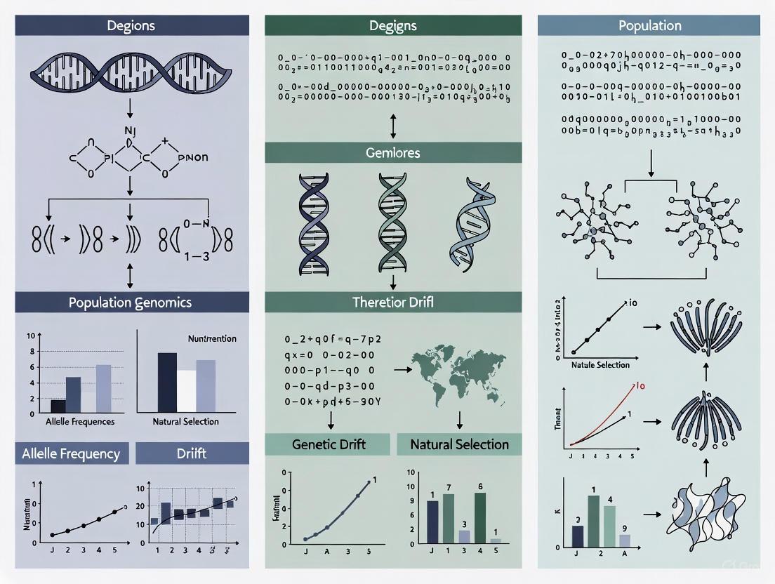
Core Principles and Genetic Variation Patterns in Populations

This technical guide delineates three foundational parameters in theoretical population genomics: theta (θ), effective population size (Ne), and exponential growth rate (R). These parameters are indispensable for quantifying genetic diversity, modeling evolutionary forces, and predicting population dynamics. The document provides rigorous definitions, methodological frameworks for estimation, and visualizes the interrelationships between these core concepts, serving as a reference for researchers and scientists in genomics and drug development.

Theta (θ): The Population Mutation Rate

Theta (θ) is a cornerstone parameter in population genetics that describes the rate of genetic variation under the neutral theory. It is fundamentally defined by the product of the effective population size and the neutral mutation rate per generation. Theta is not directly observed but is inferred from genetic data, and several estimators have been developed based on different aspects of genetic variation [1].

Primary Definitions and Estimators of θ

Estimator Name	Basis of Calculation	Formula	Key Application
Expected Heterozygosity	Expected genetic diversity under Hardy-Weinberg equilibrium [1]	H = 4_N_ₑμ (for diploids)	Provides a theoretical expectation for within-population diversity.
Pairwise Nucleotide Diversity (π)	Average number of pairwise differences between DNA sequences [1]	π = 4_N_ₑμ	Directly calculable from aligned sequence data; reflects the equilibrium between mutation and genetic drift.
Watterson's Estimator (θ_w)	Number of segregating (polymorphic) sites in a sample [1]	θw = _K / aₙ where K is the number of segregating sites and aₙ is a scaling factor based on sample size n.	Useful when full sequence data is unavailable; based on the site frequency spectrum.

Experimental Protocol: Estimating θ from Sequence Data

A standard methodology for estimating θ involves high-throughput sequencing and subsequent bioinformatic analysis [2].

• Sample Collection and DNA Extraction: Collect tissue or blood samples from a representative set of individuals from the population of interest. Extract high-molecular-weight DNA.
• Library Preparation and Sequencing: Prepare whole-genome sequencing libraries following standard protocols (e.g., Illumina). Sequence to an appropriate depth (e.g., 30x) to confidently call variants.
• Variant Calling: Map sequencing reads to a reference genome using tools like BWA or Bowtie2. Identify single nucleotide polymorphisms (SNPs) using variant callers such as GATK or SAMtools.
• Calculation of θ Estimators:
  • For Ï€: Use software like VCFtools or PopGen to calculate the average number of nucleotide differences between all possible pairs of sequences in the sample.
  • For θw: Use the same software to count the total number of segregating sites (K) in your SNP dataset and apply the formula with the appropriate sample size scaling factor _aâ‚™.

Effective Population Size (Ne)

The effective population size (Nâ‚‘) is the size of an idealized population that would experience the same rate of genetic drift or inbreeding as the real population under study [1] [3]. It is a critical parameter because it determines the strength of genetic drift, the efficiency of selection, and the rate of loss of genetic diversity. The census population size (N) is almost always larger than Nâ‚‘ due to factors such as fluctuating population size, unequal sex ratio, and variance in reproductive success [1] [4].

Key Formulations and Factors Reducing Ne

The following diagram illustrates the core concept of Nâ‚‘ and the primary demographic factors that cause it to deviate from the census size.

Table: Common Formulas for Effective Population Size (Nâ‚‘)

Scenario	Formula	Variables
Variance in Reproductive Success [1]	Nâ‚‘^(v) = (4N - 2D) / (2 + var(k))	N = census size; D = dioeciousness (0 or 1); var(k) = variance in offspring number.
Fluctuating Population Size (Harmonic Mean) [1] [4]	1 / Nₑ = (1/t) * Σ (1 / Nᵢ)	t = number of generations; Nᵢ = census size in generation i.
Skewed Sex Ratio [4]	Nₑ = (4 * Nₘ * Nƒ) / (Nₘ + Nƒ)	Nₘ = number of breeding males; Nƒ = number of breeding females.

Experimental Protocol: Estimating Ne via Temporal Method

The temporal method, which uses allele frequency changes over time, is a powerful approach to estimate Nâ‚‘ [4].

• Study Design: Collect genetic samples from the same population at two or more distinct time points (e.g., generations tâ‚€ and t₁). The number of generations between samples should be known.
• Genotyping: Genotype all samples at a set of neutral, independently segregating markers (e.g., microsatellites or SNPs).
• Allele Frequency Calculation: Calculate the allele frequencies for each marker in each temporal sample.
• Variance Calculation: For each allele, compute the variance in its frequency change between time points. The average variance across all alleles is used as var^(p) in the formula below.
• Estimation: Calculate the variance effective size using the formula [1]: Nâ‚‘^(v) = p(1-p) / (2 * var^(p)) where p is the initial allele frequency. This calculation is typically performed using specialized software like NeEstimator or MLNE, which account for sampling error and use maximum likelihood or Bayesian approaches.

Exponential Growth Rate (R)

Exponential growth occurs when a population's instantaneous rate of change is directly proportional to its current size, leading to growth that accelerates over time. The growth rate R (often denoted as r in ecology) quantifies this per-capita rate of increase [5]. While rapid exponential growth is unsustainable in the long term in natural populations, the model is crucial for describing initial phases of population expansion, bacterial culture growth, or viral infection spread [5].

Mathematical Formulations and Population Impact

The core mathematical expression for exponential growth and its key derivatives are summarized below.

Table: Key Formulas for Exponential Growth

Parameter	Formula	Variables
Discrete Growth [5]	x({}{t}) = _xâ‚€(1 + R)({}^{t})	xâ‚€ = initial population size; R = growth rate per time interval; t = number of time intervals.
Continuous Growth [5] [6]	x(t) = xâ‚€ * e({}^{R*t}	e is the base of the natural logarithm (~2.718).
Doubling Time [5]	T({}{double}) = ln(2) / _R ≈ 70 / (100*R)	The "Rule of 70" provides a quick approximation for the time required for the population to double in size.

The following diagram illustrates how exponential growth influences genomic diversity, a key consideration in population genomic models.

Experimental Protocol: Inferring Historical Growth from Genetic Data

Demographic history, including periods of exponential growth, can be inferred from genomic data using coalescent-based models [1].

• Data Generation: Obtain whole-genome sequence data from a random sample of individuals from the population. High-quality, high-coverage data is preferred.
• Site Frequency Spectrum (SFS) Construction: Calculate the SFS, which is a histogram of allele frequencies in the sample. This spectrum summarizes the proportion of sites with derived alleles found in 1, 2, 3, ..., n-1 of the n chromosomes.
• Model Selection and Fitting: Use software such as ∂a∂i (for allele frequency data) or BEAST (for phylogenetic trees) to fit a demographic model that includes an exponential growth parameter (R or a related parameter like growth rate g). The software compares the observed SFS to SFSs generated under different models and parameters.
• Parameter Estimation: The fitting algorithm (e.g., maximum likelihood or Bayesian inference) will estimate the value of R that best explains the observed genetic data, along with other parameters like the timing of the growth and the initial population size.

The Scientist's Toolkit: Key Research Reagents and Solutions

Table: Essential Materials for Population Genomic Experiments

Reagent / Tool	Function in Research
High-Fidelity DNA Polymerase	Critical for accurate PCR amplification during library preparation for sequencing and genotyping of molecular markers like microsatellites and SNPs [2].
Whole-Genome Sequencing Kit	(e.g., Illumina NovaSeq). Provides the raw sequence data required for estimating θ, inferring demography, and calling variants for Nₑ estimation [2].
SNP Genotyping Array	A cost-effective alternative to WGS for scoring hundreds of thousands to millions of SNPs across many individuals, useful for estimating Nâ‚‘ and genetic diversity [2].
Bioinformatics Software (e.g., GATK, VCFtools, ∂a∂i, BEAST)	Software suites for variant calling, data quality control, and demographic inference. They are essential for transforming raw sequence data into estimates of θ, Nₑ, and R [1] [2].
Tin tetrabutanolate	Tin Tetrabutanolate|CAS 14254-05-8|Supplier
(S)-(-)-Nicotine-15N	(S)-(-)-Nicotine-15N|High-Purity Isotope for Research

In the field of theoretical population genomics, understanding the processes that shape the distribution of genetic variation is fundamental. Two predominant models explaining patterns of genetic differentiation are Isolation by Distance (IBD) and Isolation by Environment (IBE). IBD describes a pattern where genetic differentiation between populations increases with geographic distance due to the combined effects of limited dispersal and genetic drift [7]. In contrast, IBE describes a pattern where genetic differentiation increases with environmental dissimilarity, independent of geographic distance, often as a result of natural selection against migrants or hybrids adapted to different environmental conditions [8]. Disentangling the relative contributions of these processes is crucial for understanding evolutionary trajectories, local adaptation, and for informing conservation strategies [9] [10]. This guide provides a technical overview of the theoretical foundations, methodologies, and applications of IBD and IBE for researchers and scientists.

Theoretical Foundations and Prevalence

Core Concepts and Definitions

Isolation by Distance (IBD) is a neutral model grounded in population genetics theory. It posits that gene flow is geographically limited, leading to a positive correlation between genetic differentiation and geographic distance. This pattern arises from the interplay of localized dispersal and genetic drift, which creates a genetic mosaic across the landscape [7]. The model was initially formalized by Sewall Wright, who showed that limited dispersal leads to genetic correlations among individuals based on their spatial proximity.

Isolation by Environment (IBE) is a non-neutral model that emphasizes the role of environmental heterogeneity in driving genetic divergence. IBE occurs when gene flow is reduced between populations inhabiting different environments, even if they are geographically close. This can result from several mechanisms, including:

• Natural selection against maladapted immigrants.
• Biased dispersal toward familiar environments.
• Natural or sexual selection against hybrids [8]. IBE can affect both adaptive loci and, through processes like genetic hitchhiking, neutral loci across the genome [9].

Relative Prevalence of IBD and IBE

A survey of 70 studies found that IBE is a common driver of genetic differentiation, underscoring the significant role of environmental selection in shaping population structure [11].

Table 1: Prevalence of Isolation Patterns across Studies

Pattern of Isolation	Prevalence in Studies (%)	Brief Description
Isolation by Environment (IBE)	37.1%	Genetic differentiation is primarily driven by environmental differences [11].
Both IBE and IBD	37.1%	Both geographic distance and environment contribute significantly to genetic differentiation [11].
Isolation by Distance (IBD)	20.0%	Genetic differentiation is primarily driven by geographic distance [11].
Counter-Gradient Gene Flow	10.0%	Gene flow is highest among dissimilar environments, a potential "gene-swamping" scenario [11].

The combined data shows that 74.3% of studies exhibited significant IBE patterns, suggesting it is a predominant force in nature and refuting the idea that gene swamping is a widespread phenomenon [11].

Methodological Approaches for Disentangling IBD and IBE

Experimental Design and Data Collection

Robust testing for IBD and IBE requires data on population genetics, geographic locations, and environmental variables.

• Genetic Data: Studies commonly use genome-wide single nucleotide polymorphisms (SNPs) [8] or other molecular markers like inter-simple sequence repeats (ISSRs) [9] to estimate genetic differentiation.
• Geographic Data: Precise geographic coordinates for all sampled populations are essential for calculating geographic distance matrices.
• Environmental Data: Climatic and edaphic variables (e.g., precipitation seasonality, temperature, soil pH) are obtained from field measurements or geographic information systems (GIS) [9] [8].

Statistical Frameworks and Analysis

The following statistical protocols are used to partition the effects of IBD, IBE, and other processes.

Protocol 1: Partial Mantel Tests and Maximum Likelihood Population Effects (MLPE) Models

• Purpose: To test the correlations between genetic distance, geographic distance, and environmental distance while controlling for the covariance between predictors.
• Procedure:
  • Compute pairwise matrices for genetic distance (e.g., ( F_{ST} )), geographic distance (Euclidean or resistance-based), and environmental distance (e.g., Euclidean distance of standardized climate variables).
  • Perform a partial Mantel test to assess the correlation between genetic and environmental distance while controlling for geographic distance, and vice versa.
  • Use MLPE models, a linear mixed-modeling approach, to compare the support for IBD, IBE, and IBR (Isolation by Resistance) models, which account for non-independence of pairwise data [9].
• Application: This method identified winter and summer precipitation as the main drivers of genetic differentiation in Ammopiptanthus mongolicus, supporting a primary IBE pattern [9] [12].

Protocol 2: Variance Partitioning via Redundancy Analysis (RDA)

• Purpose: To quantify the unique and shared contributions of geographic distance (IBD), environmental factors (IBE), and landscape barriers (IBB) to genetic variation.
• Procedure:
  • Perform data preparation and compute pairwise genetic distance matrices from neutral genetic markers.
  • Define predictor variable groups: geographic distances, environmental distances, and resistance distances.
  • Run a series of RDAs with the genetic data as the response variable and the distance matrices as predictors.
  • Calculate the adjusted ( R^2 ) for each set of predictors to partition the variance into unique and shared components [10].
• Application: This approach revealed that for the plains pocket gopher (Geomys bursarius), a major river acted as a barrier explaining the most genetic variation (IBB), while geographic distance (IBD) was most important for a subspecies, and soil properties contributed a smaller, unique effect (IBE) [10].

Figure 1: A generalized workflow for designing studies and analyzing data to distinguish between Isolation by Distance (IBD) and Isolation by Environment (IBE).

Research Reagent and Computational Toolkit

A successful study requires both wet-lab reagents for genetic data generation and dry-lab computational tools for analysis.

Table 2: Essential Research Toolkit for IBD/IBE Studies

Category/Item	Specific Examples	Function/Application
Molecular Markers
Genome-wide SNPs	[8]	High-resolution genotyping for estimating genetic diversity and differentiation.
Microsatellites	[10]	Co-dominant markers useful for population-level studies.
ISSR (Inter-Simple Sequence Repeats)	[9]	Dominant, multilocus markers for assessing genetic variation.
Software for Analysis
PLINK	[13]	Whole-genome association and population-based linkage analyses; includes IBD detection.
GERMLINE	[13]	Efficient, linear-time detection of IBD segments in pairs of individuals.
BEAGLE/RefinedIBD	[13]	Detects IBD segments using a hashing method and evaluates significance via likelihood ratio.
R packages (e.g., vegan, adegenet)	[9] [8] [10]	Statistical environment for performing Mantel tests, RDA, and other spatial genetic analyses.
Ned-K	Ned-K, MF:C31H31N5O3, MW:521.6 g/mol	Chemical Reagent
ATTO488-ProTx-II		ATTO488-ProTx-II is a fluorescently labeled, high-affinity blocker for Nav1.7 channels. This product is for research use only and is not intended for diagnostic or therapeutic applications.

Case Studies in Plants and Animals

Plant Systems

Case Study: Ammopiptanthus mongolicus

• Background: This endangered desert shrub was previously thought to exhibit IBD.
• Methods: Researchers used ISSR markers on 10 populations and analyzed data with partial Mantel tests and MLPE models.
• Findings: Genetic differentiation was primarily driven by climate differences (IBE), specifically summer and winter precipitation, rather than geographic distance (IBD). This led to a conservation recommendation focused on collecting germplasm from differentiated populations rather than creating connectivity corridors [9] [12].

Case Study: Arabidopsis thaliana

• Background: A model organism used to study genetic structure across the Iberian Peninsula.
• Methods: Analysis of 1772 individuals from 278 populations using genome-wide SNPs.
• Findings: Both IBD and IBE were significant drivers of genetic differentiation, with precipitation seasonality and topsoil pH being key environmental factors. The relative importance of these drivers varied among distinct genetic clusters within the region [8].

Animal Systems

Case Study: Plains Pocket Gopher (Geomys bursarius)

• Background: A subterranean rodent with a wide distribution across the Great Plains.
• Methods: Variance partitioning with microsatellite data was used to separate the effects of IBB, IBD, and IBE.
• Findings: At the species level, a major river (IBB) was the strongest isolating factor. For the subspecies G. b. illinoensis, IBD was the dominant pattern. IBE, associated with soil sand percent and color (likely related to burrowing costs and crypsis), explained a smaller but significant portion of genetic variance [10].

Figure 2: A conceptual diagram showing the primary evolutionary forces and their mechanisms behind IBD and IBE, with example outcomes from key case studies.

Implications for Conservation and Management

Identifying whether IBD or IBE is the dominant pattern has direct, and often divergent, implications for conservation policy and management.

• When IBE is Dominant: Conservation efforts should prioritize preserving genetic diversity across different environmental gradients. For A. mongolicus, this meant that collecting germplasm resources from genetically differentiated populations was a more effective strategy than establishing corridors to enhance gene flow [9]. This "several-small" approach conserves locally adapted genotypes.

• When IBD is Dominant: Conservation should focus on maintaining landscape connectivity to facilitate natural gene flow between neighboring populations. This aligns with a "single-large" strategy, as genetic diversity is maintained through proximity and gene flow [9] [10].

• Integrated Management: Many systems, like A. thaliana and the pocket gopher, show hierarchical structuring where different processes dominate at different spatial scales [8] [10]. Management must therefore be scale-aware, considering major barriers (IBB) at a regional scale while also addressing fine-scale environmental adaptation (IBE) and dispersal limitation (IBD).

Demographic processes are fundamental forces shaping the genetic architecture of populations. Theoretical population genomics relies on models that integrate these demographic forces—bottlenecks, expansions, and genetic drift—to interpret patterns of genetic variation and make inferences about a population's history [14]. These forces directly affect key genetic parameters, including the loss of genetic diversity, increased homozygosity, and the accumulation of deleterious mutations, which can reduce a population's evolutionary potential and its ability to adapt to environmental change [15]. Understanding these impacts is crucial not only for conservation biology and evolutionary studies but also for the design of robust genetic association studies in drug development, where unrecognized population structure can confound the identification of genuine disease-susceptibility genes [14]. This whitepaper provides a technical guide to the mechanisms, measurement, and consequences of these demographic events, framed within contemporary research in theoretical population genomics.

Core Concepts and Quantitative Genetic Foundations

Genetic Drift, Effective Population Size, and Variance

Genetic drift describes the random fluctuation of allele frequencies in a population over generations. Its intensity is inversely proportional to the effective population size (Ne), a key parameter in population genetics that determines the rate of loss of genetic diversity and the efficacy of selection. The fundamental variance in allele frequency change due to genetic drift from one generation to the next is given by:

σ²_Δq = pq / 2N_e

where p and q are allele frequencies [16]. This equation highlights that smaller populations experience stronger drift, leading to rapid fixation or loss of alleles and a consequent reduction in heterozygosity at a rate of 1/(2Ne) per generation.

Partitioning Genetic Variance

In quantitative genetics, the genetic variance (σ²G) of a trait can be partitioned into additive (σ²A) and dominance (σ²D) components, expressed as σ²G = σ²A + σ²D [16]. The additive genetic variance is the primary determinant of a population's immediate response to selection and is therefore critical for predicting evolutionary outcomes. Demographic events drastically alter these variance components. The additive genetic variance is a function of allele frequencies (p, q) and the average effect of gene substitution (α), defined as σ²A = 2pqα² [16]. Population bottlenecks and expansions cause rapid shifts in allele frequencies, directly impacting σ²A and, consequently, the evolutionary potential of a population.

Demographic Events: Mechanisms and Genetic Consequences

Population Bottlenecks

A population bottleneck is a sharp, often temporary, reduction in population size. The severity of a bottleneck is determined by its duration and the minimum number of individuals, which dictates the extent of genetic diversity loss and the strength of genetic drift [17] [15].

• Mechanism and Genetic Consequences: During a bottleneck, the small number of surviving individuals represents only a small fraction of the original population's gene pool. This leads to a sudden drop in heterozygosity and the possible loss of rare alleles. Following the bottleneck, genetic diversity remains low and can only be restored slowly through mutation or via gene flow from other populations [15]. Furthermore, the increased rate of inbreeding in small populations can lead to inbreeding depression, reducing fitness [15].
• Examples from Research:
  • Northern Elephant Seals: Hunted to a mere ~20 individuals in the 1890s. Despite a recovery to over 30,000 individuals, they exhibit drastically reduced genetic variation compared to closely related species that did not experience such intense hunting [17] [15].
  • Sophora moorcroftiana: Genomic analysis of this Tibetan shrub revealed distinct subpopulations that underwent severe bottlenecks. The subpopulation P1 (Gongbu Jiangda County) showed the lowest genetic diversity (Ï€ = 1.1 × 10⁻⁴) and the smallest effective population size, a clear genetic signature of a past bottleneck [18].

Table 1: Quantified Genetic Consequences of Documented Population Bottlenecks

Species	Bottleneck Severity	Key Genetic Metric	Post-Bottleneck Value	Citation
Northern Elephant Seal	Reduced to ~20 individuals	Genetic Diversity (vs. Southern seals)	Much lower	[17] [15]
Sophora moorcroftiana (P1)	Severe bottleneck	Nucleotide Diversity (π)	1.1 × 10⁻⁴	[18]
Wollemi Pine	< 50 mature individuals	Genetic Diversity	Nearly undetectable	[15]
Greater Prairie Chicken	100 million to 46 (in Illinois)	Genetic Decline (DNA analysis)	Steep decline	[15]

Founder Effects

A founder effect is a special case of a bottleneck that occurs when a new population is established by a small number of individuals from a larger source population. The new colony is characterized by reduced genetic variation and a gene pool that is a non-representative sample of the original population [17].

• Mechanism and Genetic Consequences: The founding group carries only a small, random subset of the alleles from the parent population. This can lead to the rapid emergence of rare diseases in the new population if the founders by chance carry deleterious alleles. An iconic example is the Afrikaner population in South Africa, which has an unusually high frequency of the gene causing Huntington's disease due to its high prevalence among the few original Dutch colonists [17].

Population Expansions

Population expansions occur when a population experiences a significant increase in size, often following a bottleneck or after colonizing new habitats. While expansions increase the absolute number of individuals and mutation supply, they leave a distinct genetic signature.

• Mechanism and Genetic Consequences: A rapid expansion from a small founder population can create a genome-wide pattern of rare, low-frequency alleles due to the influx of new mutations in the growing population. Analysis of Sophora moorcroftiana subpopulations using SMC++ analyses demonstrated that the species' demographic history was marked not only by bottlenecks but also by population expansion events, likely driven by glacial-interglacial cycles and geological events [18].

Interaction of Demography with Selection

Demographic history profoundly influences the effectiveness of natural selection. In large, stable populations, selection is efficient at removing deleterious alleles and fixing beneficial ones. In populations undergoing repeated bottlenecks or founder events, however, genetic drift can overpower selection. This can lead to the random fixation of slightly deleterious alleles, a process known as the "drift load," reducing the mean fitness of the population [15]. This is a critical consideration in conservation and biomedical genetics, as small, isolated populations may accumulate deleterious genetic variants.

The following diagram illustrates the logical relationship between different demographic events and their primary genetic consequences.

Diagram 1: Logical flow from demographic events to genetic consequences. Bottlenecks and founder effects trigger strong genetic drift and reduce Ne, leading to a cascade of negative genetic outcomes.

Experimental Methodologies and Protocols

Modern population genomics employs a suite of computational and statistical tools to detect and quantify the impact of past demographic events.

Inferring Population Structure and Demography

Protocol 1: Population Genomic Analysis for Demographic Inference

• Sample Collection and Sequencing: Collect tissue samples (e.g., leaves, blood) from multiple individuals across the species' geographic range. For plants, formally identify species and deposit voucher specimens in a herbarium [18].
• Genotyping: Perform high-throughput sequencing (e.g., Whole-Genome Sequencing, Genotyping-by-Sequencing [GBS]) to generate genome-wide data. Align sequence reads to a reference genome and perform variant calling to identify single nucleotide polymorphisms (SNPs) [18].
• Population Genomic Statistics:
  • Calculate genetic diversity within populations (e.g., nucleotide diversity, Ï€).
  • Estimate genetic differentiation between populations (e.g., F-statistics, FST). The Sophora study found an average FST of 0.2477 for the most differentiated subpopulation [18].
  • Analyze population structure using algorithms like ADMIXTURE, STRUCTURE, or PCA [19].
• Demographic History Modeling:
  • Use specialized software like SMC++ to model past changes in effective population size over time, identifying periods of bottleneck and expansion [18].
  • Utilize tools like Treemix to infer historical patterns of gene flow between populations [18].

Protocol 2: Genotype-Environment Association (GEA) Analysis

• Environmental Data Collection: Gather geo-referenced environmental data (e.g., altitude, temperature, precipitation) for each sample location [18].
• Statistical Testing: Perform genotype-environment association analyses (e.g., using RDA, BayPass, or LFMM) to identify SNPs whose frequencies are significantly correlated with environmental variation [18].
• Gene Annotation: Annotate significant SNPs to identify candidate genes involved in local adaptation, which may have been targets of selection during demographic shifts. The Sophora study annotated 55 significant SNPs to 20 candidate genes [18].

Visualization and Analysis Toolkit

The complexity of genomic data necessitates advanced visualization platforms. PopMLvis is an interactive tool designed to analyze and visualize population structure using genotype data from GWAS [19]. Its functionalities include:

• Input Flexibility: Accepts raw genotype data, principal components, and admixture coefficient matrices.
• Dimensionality Reduction: Performs PCA, t-SNE, and PC-Air (which accounts for relatedness).
• Clustering and Outlier Detection: Integrates K-means, Hierarchical Clustering, and machine learning-based outlier detection.
• Interactive Visualization: Generates scatter plots, admixture bar charts, and dendrograms for publication-ready figures [19].

Table 2: Essential Research Reagents and Computational Tools for Population Genomic Studies

Item/Tool Name	Type	Primary Function in Analysis	Application Context
GBS / WGS Library Prep	Wet-lab Kit	High-throughput sequencing to generate genome-wide SNP data	Genotyping of non-model organisms [18]
Reference Genome	Data	A sequenced and annotated genome for read alignment and variant calling	Essential for accurate SNP calling and annotation [18]
VCFtools / BCFtools	Software	Filtering and manipulating variant call format (VCF) files	Pre-processing of SNP data before analysis [19]
ADMIXTURE	Software	Model-based estimation of individual ancestries from multi-locus SNP data	Inferring population structure and admixture proportions [19]
SMC++	Software	Inferring population size history from whole-genome data	Detecting historical bottlenecks and expansions [18]
R/qtl / BayPass	Software	Identifying correlations between genetic markers and environmental variables	Genotype-Environment Association (GEA) analysis [18]
PopMLvis	Web Platform	Interactive visualization of population structure results from multiple algorithms	Integrating and interpreting clustering and ancestry results [19]
BDS-I	BDS-I, MF:C210H297N57O56S6, MW:4708.37 Da	Chemical Reagent	Bench Chemicals
2-Azidoethanol-d4	2-Azidoethanol-d4, MF:C₂HD₄N₃O, MW:91.11	Chemical Reagent	Bench Chemicals

The following diagram outlines a generalized workflow for a population genomic study, from sampling to demographic inference.

Diagram 2: A workflow for population genomic analysis to infer demographic history, from sampling to synthesis.

Demographic processes—bottlenecks, expansions, and the persistent force of genetic drift—are inseparable from the patterns of genetic variation observed in natural populations. The integration of theoretical population genetics with modern genomic technologies allows researchers to reconstruct a population's history with unprecedented detail, revealing how past climatic events, geological upheavals, and human activities have shaped genomes. For drug development professionals, a rigorous understanding of these dynamics is critical. Unaccounted-for population structure can create spurious associations in genetic association studies, while a thorough characterization of demographic history can help isolate true signals of adaptive evolution and identify genetic variants underlying complex diseases. As genomic datasets grow in size and complexity, the continued refinement of demographic models and analytical tools will be essential for accurately interpreting the genetic tapestry of life.

Functional genomics provides the critical methodological bridge that connects static genomic sequences (genotype) to observable characteristics (phenotype), a central challenge in modern biology. Framed within theoretical population genomics models, this discipline leverages statistical and computational tools to understand how evolutionary processes like mutation, selection, and drift shape the genetic underpinnings of complex traits. This whitepaper details the core principles, methodologies, and analytical frameworks that empower researchers to map and characterize the functional elements of genomes, thereby illuminating the path from genetic variation to phenotypic diversity and disease susceptibility.

The relationship between genotype and phenotype is foundational to evolutionary biology and genetics. Historically, geneticists sought to understand the processing of gene expression into phenotypic design without the molecular tools available today [20]. The core challenge lies in the fact that this relationship is rarely linear; it is shaped by complex networks of gene interactions, regulation, and environmental factors. Theoretical population genomics provides the models to understand how these functional links evolve—how natural selection acts on phenotypic variation that has a heritable genetic basis, and how demographic history and genetic drift shape the architecture of complex traits.

Functional genomics addresses this by systematically identifying and characterizing the functional elements within genomes. It moves beyond correlation to causation, asking not just where genetic variation occurs, but how it alters molecular functions and, ultimately, organismal phenotypes. This guide outlines the key experimental and computational protocols that make this possible, with a focus on applications in biomedical and evolutionary research.

Methodological Foundations: Key Experimental Protocols

The following section provides detailed methodologies for key experiments that link genotype to phenotype, from data acquisition to functional validation.

Genomic Data Acquisition and Analysis Using Public Browsers

Principle: Public genome browsers are indispensable for initial genomic annotation and comparison. They provide reference genomes and annotated features (genes, regulatory elements, variants) for a wide range of species, enabling researchers to contextualize their genomic data [21].

Protocol 1: Genome Identification and Annotation via ENSEMBL

• Aim: To annotate and compare a genomic sequence of interest against a reference database.
• Method: [21]
  • Navigate to the ENSEMBL website (e.g., https://asia.ensembl.org).
  • Input the genomic sequence (e.g., from a test organism) or the name of the organism.
  • Utilize integrated tools such as BLAST or BLAT for sequence alignment.
  • Use the Variant Effect Predictor (VEP) to annotate and predict the functional consequences of genetic variants.
  • Browse the genomic landscape to identify genes, regulatory regions, and homologous sequences.
• Results: Save the annotated data for downstream analysis. The output provides a preliminary functional annotation of the genomic region.

Protocol 2: Comparative Genomics and Evolutionary Analysis via UCSC Genome Browser

• Aim: To visualize a genomic region and its evolutionary conservation across species.
• Method: [21]
  • Access the UCSC Genome Browser (https://genome.ucsc.edu).
  • Select the relevant genome assembly and input the genomic coordinates or sequence.
  • Enable comparative genomics tracks, such as conservation scores (e.g., PhastCons, PhyloP) and multiple sequence alignments.
  • Analyze the data to identify evolutionarily constrained regions, which are putative functional elements.
• Results: Save conservation scores and multiple alignment data. Highly conserved non-coding elements often indicate regulatory function.

Functional Validation via Genomic Perturbation

Principle: Establishing causality requires experimental perturbation of a genetic element and observation of the phenotypic consequence. This protocol outlines a general workflow for functional validation.

• Aim: To determine the phenotypic impact of a specific genetic variant or gene.
• Method:
  • Target Identification: Based on GWAS or QTL mapping, select a candidate gene or non-coding variant for testing.
  • Perturbation Design:
    • For coding genes: Design CRISPR-Cas9 guides for gene knockout or use RNAi for knockdown.
    • For non-coding variants: Use base-editing or prime-editing to introduce the specific allele in an isogenic background.
  • Delivery: Introduce the perturbation construct into the target cell line (e.g., via transfection) or model organism (e.g., via microinjection).
  • Phenotypic Screening: Assay for relevant phenotypic changes.
    • Molecular Phenotypes: RNA-seq (transcriptome), ATAC-seq (chromatin accessibility), proteomics.
    • Cellular Phenotypes: Cell proliferation, migration, or apoptosis assays.
    • Organismal Phenotypes: Morphological, physiological, or behavioral assessments.
• Results: A significant change in the assayed phenotype upon genetic perturbation confirms a functional link between the genotype and phenotype.

The following workflow diagram summarizes the core iterative process of linking genotype to phenotype.

The Scientist's Toolkit: Research Reagent Solutions

Successful functional genomics research relies on a suite of essential reagents and computational tools. The table below details key resources for major experimental workflows.

Table 1: Essential Research Reagents and Tools for Functional Genomics

Item/Tool Name	Function/Application	Key Features
ENSEMBL Browser [21]	Genome annotation, variant analysis, and comparative genomics.	Integrated tools like BLAST, BLAT, and the Variant Effect Predictor (VEP).
UCSC Genome Browser [21]	Visualization of genomic data and evolutionary conservation.	Customizable tracks for conservation (PhastCons), chromatin state (ENCODE), and more.
CRISPR-Cas9 System	Targeted gene knockout or editing for functional validation.	High precision and programmability for disrupting genetic elements.
RNAi Libraries	High-throughput gene knockdown screens.	Allows for systematic silencing of genes to assess phenotypic impact.
Bulk/Single-Cell RNA-seq	Profiling gene expression across samples or cell types.	Quantifies transcript abundance, identifying expression QTLs (eQTLs).
ATAC-seq	Assaying chromatin accessibility and open chromatin regions.	Identifies active regulatory elements (e.g., promoters, enhancers).
Statistical Genomics Tools [22]	Computational analysis of genomic data sets.	Provides protocols for QTL mapping, association studies, and data integration.
CYT387-azide	CYT387-azide|JAK Inhibitor Probe|Research Use Only	CYT387-azide is a functionalized JAK1/JAK2 inhibitor for synthesizing bioconjugates. For Research Use Only. Not for human or veterinary diagnosis or therapeutic use.

Data Integration and Analysis: A Quantitative Framework

Integrating data from multiple genomic layers is essential for a holistic view. The following table provides a comparative overview of key quantitative data types and their analytical interpretations within population genomics models.

Table 2: Quantitative Data Types and Their Interpretation in Functional Genomics

Data Type	Typical Measurement	Population Genomics Interpretation
Selection Strength	Composite Likelihood Ratio (e.g., CLR test)	Identifies genomic regions under recent positive or balancing selection.
Population Differentiation	FST (Fixation Index)	Highlights loci with divergent allele frequencies between populations, suggesting local adaptation.
Allele Frequency Spectrum	Tajima's D	Deviations from neutral expectations can indicate population size changes or selection.
Variant Effect	Combined Annotation Dependent Depletion (CADD) Score	Prioritizes deleterious functional variants likely to impact phenotype.
Expression Heritability	Expression QTL (eQTL) LOD Score	Quantifies the genetic control of gene expression levels.
Genetic Architecture	Number of loci & Effect Size Distribution	Informs whether a trait is controlled by few large-effect or many small-effect variants.

Analytical Framework: From Data to Biological Insight

The path from raw genomic data to a validated genotype-phenotype link requires a structured analytical pipeline. The following diagram visualizes this multi-step computational and experimental workflow, which is central to functional genomics.

Functional genomics has transformed our ability to decipher the functional code within genomes, moving from associative links to causal mechanisms underlying phenotypic variation. The integration of these approaches with theoretical population genomics models is crucial for understanding the evolutionary forces that have shaped these links. Looking ahead, the field is moving towards the widespread adoption of multiomics, which integrates data from genomics, transcriptomics, epigenetics, and proteomics [23]. This integrated approach provides a more comprehensive understanding of molecular changes and is expected to drive breakthroughs in drug development and improve patient outcomes. Furthermore, advancements in population genomics, including the collection of diverse genetic datasets and the application of whole genome sequencing in clinical diagnostics (e.g., for cancer and tuberculosis), hold transformative potential for personalized medicine [23]. As these technologies mature, they will further illuminate the intricate path from genotype to phenotype, empowering researchers and clinicians to better predict, diagnose, and treat complex diseases.

Key Models and Their Application in Genomic Selection and Drug Discovery

Genomic Selection (GS) is a revolutionary methodology in modern breeding and genetic research that enables the prediction of an individual's genetic merit based on dense genetic markers covering the entire genome. First conceptualized by Meuwissen, Hayes, and Goddard in 2001, GS represents a fundamental shift from marker-assisted selection (MAS) by utilizing all marker information simultaneously, thereby capturing both major and minor gene effects contributing to complex traits [24] [25]. This approach has become standard practice in major dairy cattle, pig, and chicken breeding programs worldwide, providing multiple quantifiable benefits to breeders, producers, and consumers [26]. The core principle of GS involves first estimating marker effects based on genotypic and phenotypic values of a training population, then applying these estimated effects to compute genomic estimated breeding values (GEBVs) for selection candidates in a test population having only genotypic information [24]. This allows for selection decisions at an early growth stage, significantly reducing breeding time and costs, particularly for traits that express later in life or are costly to phenotype [24].

The accuracy of GEBVs is paramount to the success of genomic predictions and is influenced by several factors including trait heritability, marker density, quantitative trait loci (QTL) number, linkage disequilibrium between QTL and associated markers, size of the reference population, and genetic relationship between reference and test populations [24] [27]. With the advent of low-cost genotyping technologies such as single nucleotide polymorphism (SNP) arrays and genotyping by sequencing, GS has become increasingly accessible, enabling more efficient breeding programs across animal and plant species [24].

Theoretical Foundations of Genomic Selection Models

Statistical Framework

Genomic selection methods can be broadly classified into parametric, semi-parametric, and non-parametric approaches [24] [27]. Parametric methods assume specific distributions for genetic effects and include BLUP (Best Linear Unbiased Prediction) alphabets and Bayesian alphabets. Semi-parametric methods include approaches like reproducing kernel Hilbert space (RKHS), while non-parametric methods comprise mostly machine learning techniques [24]. The fundamental statistical model for genomic prediction can be represented as:

y = 1μ + Xg + e

Where y is the vector of phenotypes, μ is the overall mean, X is the matrix of genotype indicators, g is the vector of random marker effects, and e is the vector of residual errors [28]. In this model, the genomic estimated breeding value (GEBV) for an individual is calculated as the sum of all marker effects according to its marker genotypes [28].

The differences between various GS methods primarily lie in the assumptions regarding the distribution of marker effects and how these effects are estimated [24]. These methodological differences lead to varying performance across traits with different genetic architectures, making the selection of an appropriate statistical model crucial for accurate genomic prediction.

Key Methodological Distinctions

The BLUP and Bayesian approaches differ fundamentally in their treatment of marker effects. BLUP alphabets assume all markers contribute to trait variability, with marker effects following a normal distribution, implying that many QTLs govern the trait, each with small effects [24]. In contrast, Bayesian methods assume only a limited number of markers have effects on trait variance, with different prior distributions specified for different Bayesian models [24]. Additionally, BLUP methods assign equal variance to all markers, while Bayesian methods assign different weights to different markers, allowing for variable contributions to the genetic variance [24].

Table 1: Core Methodological Differences Between BLUP and Bayesian Approaches

Feature	BLUP Alphabets	Bayesian Alphabets
Method Type	Linear parametric	Non-linear parametric
Marker Effect Assumption	All markers have effects	Limited number of markers have effects
Marker Effect Distribution	Normal distribution	Various prior distributions depending on method
Variance Treatment	Common variance for all marker effects	Marker-specific variances (except BayesC and BRR)
Estimation Method	Linear mixed model with spectral factorization	Markov chain Monte Carlo (MCMC) with Gibbs sampling
Computational Efficiency	High	Variable, generally lower than BLUP

G-BLUP (Genomic Best Linear Unbiased Prediction)

Theoretical Basis and Methodology

G-BLUP is a linear parametric method that has gained widespread adoption due to its computational efficiency and similarity to traditional BLUP methods [29]. In G-BLUP, the genomic relationship matrix (G-matrix) derived from markers replaces the pedigree-based relationship matrix (A-matrix) used in traditional BLUP [29]. The model can be represented as:

y = 1μ + Zu + e

Where y is the vector of phenotypes, μ is the overall mean, Z is an incidence matrix relating observations to individuals, u is the vector of genomic breeding values with variance-covariance matrix Gσ²_u, and e is the vector of residual errors [28]. The G matrix, or realized relationship matrix, is constructed using genotypes of all markers according to the method described by VanRaden (2008) [28].

The primary advantage of G-BLUP lies in its computational efficiency, as it avoids the need to estimate individual marker effects directly [29]. Instead, it focuses on estimating the total genomic value of each individual, making it particularly suitable for applications with large datasets. The method assumes that all markers contribute equally to the genetic variance, which works well for traits influenced by many genes with small effects [24].

Experimental Implementation

Implementing G-BLUP requires several key steps. First, quality control of genotype data is performed, including filtering based on minor allele frequency (typically <5%), call rate, and Hardy-Weinberg equilibrium [27]. The genomic relationship matrix G is then constructed using the remaining markers. Different algorithms exist for constructing G, with VanRaden's method being among the most popular [28].

Variance components are estimated using restricted maximum likelihood (REML), which provides unbiased estimates of the genetic and residual variances [28]. These variance components are then used to solve the mixed model equations to obtain GEBVs for all genotyped individuals. The accuracy of GEBVs is typically evaluated using cross-validation approaches, where the data is partitioned into training and validation sets, and the correlation between predicted and observed values in the validation set is calculated [24] [27].

In practice, G-BLUP has been extensively applied to actual datasets to evaluate genomic prediction accuracy across various species and traits [24]. Its implementation has been facilitated by the development of specialized software packages that efficiently handle the computational demands of large-scale genomic analyses.

Bayesian Alphabet Methods

Theoretical Foundations

Bayesian methods for genomic selection represent a different philosophical approach from BLUP methods, treating all markers as random effects and offering flexibility through the use of different prior distributions [24]. The Bayesian framework allows for the incorporation of prior knowledge about the distribution of marker effects, which is particularly valuable for traits with suspected major genes [24]. The general Bayesian model for genomic selection can be represented as:

y = 1μ + Xg + e

Where the key difference lies in the specification of prior distributions for the marker effects g [28]. Unlike BLUP methods that assume a homogeneous variance structure across all markers, Bayesian methods allow for heterogeneous variances, enabling some markers to have larger effects than others [24].

The Bayesian approach employs Markov chain Monte Carlo (MCMC) methods, particularly Gibbs sampling, to estimate the posterior distributions of parameters [24]. This computational intensity represents both a strength and limitation of Bayesian methods - while allowing for more flexible modeling of genetic architecture, it requires substantial computational resources, especially for large datasets [24].

Key Bayesian Methods

BayesA

BayesA assumes that all markers have an effect, but each has a different variance [24]. The prior distribution for marker effects follows a scaled t-distribution, which has heavier tails than the normal distribution, allowing for larger marker effects [24]. This makes BayesA particularly suitable for traits influenced by a few genes with relatively large effects. The method requires specifying degrees of freedom and scale parameters for the prior distribution, which influence the extent of shrinkage applied to marker effects.

BayesB

BayesB extends BayesA by introducing a mixture distribution that allows some markers to have zero effects [24]. It assumes that a proportion π of markers have no effect on the trait, while the remaining markers have effects with different variances [24]. This method is particularly useful for traits with a known sparse genetic architecture, where only a small number of markers are expected to have substantial effects. The proportion π can be treated as either a fixed parameter or estimated from the data.

BayesC

BayesC modifies the BayesB approach by assuming that markers with non-zero effects share a common variance [24]. Similar to BayesB, it assumes that only a fraction of markers have effects on the trait, but unlike BayesB, these effects are drawn from a distribution with common variance [24]. This method represents a compromise between the sparse model of BayesB and the dense model of BayesA, reducing the number of parameters that need to be estimated.

Bayesian LASSO

Bayesian LASSO (Least Absolute Shrinkage and Selection Operator) uses a double exponential (Laplace) prior for marker effects, which induces stronger shrinkage of small effects toward zero compared to normal priors [24]. This approach is particularly effective for variable selection in high-dimensional problems, as it tends to produce sparse solutions where many marker effects are estimated as zero. The Bayesian implementation of LASSO allows for estimation of the shrinkage parameter within the model, avoiding the need for cross-validation.

Bayesian Ridge Regression

Bayesian Ridge Regression (BRR) assumes that all marker effects have a common variance and follow a Gaussian distribution [24]. This results in shrinkage of estimates similar to ridge regression, with all effects shrunk toward zero to the same degree. BRR is most appropriate for traits governed by many genes with small effects, as it does not allow for potentially large effects at individual loci.

Table 2: Comparison of Bayesian Alphabet Methods

Method	Marker Effects	Variance Structure	Prior Distribution	Best Suited For
BayesA	All markers have effects	Marker-specific variances	Scaled t-distribution	Traits with few genes of moderate to large effects
BayesB	Some markers have zero effects	Marker-specific variances for non-zero effects	Mixture distribution with point mass at zero	Traits with sparse genetic architecture
BayesC	Some markers have zero effects	Common variance for non-zero effects	Mixture distribution with point mass at zero	Balanced approach for various genetic architectures
Bayes LASSO	All markers have effects, but many shrunk to zero	Implicitly marker-specific through shrinkage	Double exponential (Laplace)	Variable selection in high-dimensional settings
Bayes Ridge Regression	All markers have effects	Common variance for all effects	Gaussian distribution	Highly polygenic traits

Experimental Protocols and Methodological Comparisons

Standard Evaluation Framework

To ensure fair comparison between different genomic selection methods, researchers have established standardized evaluation protocols. These typically involve fivefold cross-validation with 100 replications to measure genomic prediction accuracy using Pearson's correlation coefficient between GEBVs and observed phenotypic values [24]. The bias of GEBV estimation is measured as the regression of observed values on predicted values [24].

The general workflow for comparative studies involves several key steps. First, datasets are divided into training and validation populations, with the validation population comprising individuals with genotypes but no phenotypic records [28]. Each method is then applied to the training population to estimate marker effects or genomic values. These estimates are used to predict GEBVs for the validation population, and accuracy is assessed by comparing predictions to true breeding values when available or through cross-validation [24] [28].

Diagram 1: Experimental workflow for comparing genomic selection methods

Performance Across Genetic Architectures

Comprehensive studies comparing three BLUP and five Bayesian methods using both actual and simulated datasets have revealed important patterns in method performance relative to trait genetic architecture [24]. Bayesian alphabets generally perform better for traits governed by a few genes/QTLs with relatively larger effects, while BLUP alphabets (GBLUP and CBLUP) exhibit higher genomic prediction accuracy for traits controlled by several small-effect QTLs [24]. Additionally, Bayesian methods perform better for highly heritable traits and perform at par with BLUP methods for other traits [24].

The performance differences between methods can be substantial. In one study comparing GBLUP and Bayesian methods, the correlations between GEBVs by different methods ranged from 0.812 (GBLUP and BayesCÏ€) to 0.997 (TABLUP and BayesB), with accuracies of GEBVs (measured as correlations between true breeding values and GEBVs) ranging from 0.774 (GBLUP) to 0.938 (BayesCÏ€) [28]. These results highlight the importance of matching method selection to the expected genetic architecture of the target trait.

Table 3: Performance Comparison Across Different Genetic Architectures

Genetic Architecture	Heritability	Best Performing Methods	Key Findings
Few QTLs with large effects	High	BayesB, BayesA, Bayesian LASSO	Bayesian methods significantly outperform GBLUP by capturing major effect QTLs
Many QTLs with small effects	Moderate to High	GBLUP, Bayes Ridge Regression	BLUP methods perform similarly or better than Bayesian approaches
Mixed architecture	Variable	BayesC, Bayesian LASSO	Flexible methods that balance sparse and dense models perform best
Low heritability traits	Low	Compressed BLUP (cBLUP)	Specialized BLUP variants outperform standard methods for low heritability

Bias and Reliability Assessment

Beyond prediction accuracy, the bias of GEBV estimation is an important consideration in method selection. Studies have identified GBLUP as the least biased method for GEBV estimation [24]. Among Bayesian methods, Bayesian Ridge Regression and Bayesian LASSO were found to be less biased than other Bayesian alphabets [24]. Bias is typically measured as the regression of true breeding values on GEBVs, with values closer to 1.0 indicating less bias [28].

The reliability of predictions, particularly in the context of breeding applications, is another critical metric. Not separating dominance effects from additive effects has been shown to decrease accuracy and reliability while increasing bias of predicted genomic breeding values [30]. Including dominance genetic effects in models generally increases the efficiency of genomic selection, regardless of the statistical method used [30].

Advanced Extensions and Methodological Innovations

Expanding the BLUP Alphabet

Recent research has focused on expanding the BLUP alphabet to maintain computational efficiency while improving prediction accuracy across diverse genetic architectures. Two notable innovations include SUPER BLUP (sBLUP) and compressed BLUP (cBLUP) [29]. sBLUP substitutes all available markers with estimated quantitative trait nucleotides (QTNs) to derive kinship, while cBLUP compresses individuals into groups based on kinship and uses groups as random effects instead of individuals [29].

These expanded BLUP methods offer flexibility for evaluating a variety of traits covering a broadened realm of genetic architectures. For traits controlled by small numbers of genes, sBLUP can outperform Bayesian LASSO, while for traits with low heritability, cBLUP outperforms both GBLUP and Bayesian LASSO methods [29]. This development represents an important advancement in making BLUP approaches more adaptable to different genetic architectures while maintaining computational advantages.

Integration of Dominance and Epistatic Effects

Traditional GS models have primarily focused on additive genetic effects, but non-additive effects can contribute significantly to trait variation. Recent methodological advances have incorporated dominance and epistatic effects into genomic prediction models [30]. Studies have shown that not separating dominance effects from additive effects leads to decreased accuracy and reliability and increased bias of predicted genomic breeding values [30].

Bayesian methods generally show better performance than GBLUP for traits with non-additive genetic architecture, exhibiting higher prediction accuracy and reliability with less bias [30]. The inclusion of dominance effects is particularly important for traits where heterosis or inbreeding depression are significant factors, such as in crossbreeding systems or for fitness-related traits.

Essential Research Reagents

Table 4: Key Research Reagents and Resources for Genomic Selection Studies

Resource Type	Specific Examples	Function/Application
Genotyping Platforms	Illumina SNP arrays, Affymetrix Axiom arrays, Genotyping-by-Sequencing (GBS)	Generate dense genetic marker data for training and validation populations
Reference Genomes	Species-specific reference assemblies (e.g., ARS-UCD1.2 for cattle, GRCm39 for mice)	Provide framework for aligning sequences and assigning marker positions
Biological Samples	DNA from blood, tissue, or semen samples (animals), leaf tissue (plants)	Source material for genotyping and establishing training populations
Phenotypic Databases	Historical breeding records, field trial data, clinical measurements	Provide phenotypic measurements for model training and validation
Software Packages	GAPIT, BGLR, DMU, ASReml, BLUPF90	Implement various GS methods and statistical analyses

Computational Implementation

The implementation of genomic selection methods requires specialized software tools. The R package BGLR (Bayesian Generalized Linear Regression) provides comprehensive implementations of Bayesian methods, allowing users to specify different prior distributions for marker effects [30]. For BLUP-based approaches, the Genome Association and Prediction Integrated Tool (GAPIT) implements various BLUP alphabet methods including the newly developed sBLUP and cBLUP [29].

Computational requirements vary significantly between methods. GBLUP and related BLUP methods are generally the fastest, while Bayesian methods requiring MCMC sampling are computationally intensive [24] [30]. Boosting algorithms have been identified as among the slowest methods for genomic breeding value prediction [30]. This computational efficiency differential is an important practical consideration when selecting methods for large-scale applications.

The comparison between G-BLUP and Bayesian alphabet methods reveals a complex landscape where no single method universally outperforms others across all scenarios. The optimal choice depends critically on the genetic architecture of the target trait, with Bayesian methods generally superior for traits governed by few genes of large effect, and G-BLUP performing well for highly polygenic traits [24]. Recent expansions to the BLUP alphabet, such as sBLUP and cBLUP, show promise in bridging this performance gap while maintaining computational efficiency [29].

Future developments in genomic selection will likely focus on integrating multi-omics data, including transcriptomics, proteomics, and epigenomics, to improve prediction accuracy [31]. The incorporation of artificial intelligence and machine learning approaches represents another frontier, with tools like Google's DeepVariant already showing improved variant calling accuracy [31]. As sequencing technologies continue to advance and costs decrease, the application of whole-genome sequence data in genomic selection promises to further enhance prediction accuracy by potentially capturing causal variants directly.

The ongoing challenge for researchers and breeders remains the appropriate matching of methods to specific applications, considering both statistical performance and practical constraints. As genomic selection continues to evolve, the development of adaptable, computationally efficient methods that perform well across diverse genetic architectures will be crucial for maximizing genetic gain in breeding programs and advancing our understanding of complex trait genetics.

Identity-by-Descent (IBD) Detection in High-Recombining Genomes

Identity-by-Descent (IBD) refers to genomic segments inherited by two or more individuals from a common ancestor without recombination [13]. These segments are "maximal," meaning they are bounded by recombination events on both ends [13]. In theoretical population genomics, IBD analysis is a cornerstone for inferring demographic history, detecting natural selection, estimating effective population size (Ne), and understanding fine-scale population structure [32] [33].

The reliability of these inferences is highly dependent on the accurate detection of IBD segments. This presents a significant challenge when studying organisms with high recombination rates, such as the malaria parasite Plasmodium falciparum (P. falciparum). In these genomes, high recombination relative to mutation leads to low marker density per genetic unit, which can severely compromise IBD detection accuracy [32] [34] [33]. This technical guide explores the specific challenges of IBD detection in high-recombining genomes, provides benchmarking data for contemporary tools, outlines optimized experimental protocols, and discusses implications for genomic surveillance and drug development.

The Challenge of High-Recombining Genomes

High-recombining genomes like P. falciparum exhibit evolutionary parameters that diverge significantly from the human genome, for which many IBD detection tools were originally designed. The core of the challenge lies in the balance between recombination and mutation rates.

P. falciparum recombines approximately 70 times more frequently per unit of physical distance than humans [32] [33]. However, it shares a similar mutation rate with humans, on the order of 10⁻⁸ per base pair per generation [32] [33]. This high recombination-to-mutation rate ratio results in a drastically reduced number of common variants, such as Single Nucleotide Polymorphisms (SNPs), per centimorgan (cM). While large human whole-genome sequencing datasets typically provide millions of common biallelic SNPs, P. falciparum datasets only contain tens of thousands [32] [33]. Consequently, the per-cM SNP density in P. falciparum can be two orders of magnitude lower than in humans (approximately 25 SNPs/cM vs. 1,660 SNPs/cM) [33], often providing insufficient information for accurate IBD segment detection.

This low marker density per genetic unit disproportionately affects the detection of shorter IBD segments, which are critical for analyzing older relatedness and complex demographic histories. Performance degradation manifests as elevated false negative rates (failure to detect true IBD segments) and/or false positive rates (erroneous inference of non-existent segments) [32] [33].

Benchmarking IBD Detection Tools

A unified benchmarking framework for high-recombining genomes has revealed that the performance of IBD callers varies significantly under low SNP density conditions. The following table summarizes the key characteristics and performance of several commonly used and recently developed tools.

Table 1: Benchmarking of IBD Detection Tools for High-Recombining Genomes

Tool	Underlying Method	Key Features	Performance in High Recombination
hmmIBD / hmmibd-rs [32] [35]	Probabilistic (Hidden Markov Model)	Designed for haploid genomes; robust to low SNP density.	Superior accuracy for shorter segments; provides less biased Ne estimates; low false positive rate [32] [34].
isoRelate [33]	Probabilistic (Hidden Markov Model)	Designed for Plasmodium species.	Better IBD quality with lower marker densities; suffers from high false negative rates for shorter segments [33].
Refined IBD [33]	Identity-by-State-based	Originally designed for human genomes.	High false negative rates for shorter segments in P. falciparum-like genomes [33].
hap-IBD [33]	Identity-by-State-based	Scales well to large sample sizes and genomes.	High false negative rates for shorter segments in P. falciparum-like genomes [33].
phased IBD [33]	Identity-by-State-based	Recent advancement in IBD detection.	High false negative rates for shorter segments in P. falciparum-like genomes [33].
KinSNP [36]	IBD segment-based	Used for human identification in forensic contexts.	Validated for human data; accuracy maintained with up to 75% simulated missing data, but sensitive to sequence errors [36].

The benchmarking results indicate that hmmIBD consistently outperforms other methods in the context of high-recombining genomes, particularly for quality-sensitive downstream analyses like effective population size estimation [32] [34]. Its probabilistic framework, specifically tailored for haploid genomes, makes it more robust to the challenges of low SNP density.

Table 2: Quantitative Benchmarking Results from Simulated P. falciparum-like Genomes

Performance Metric	hmmIBD	isoRelate	Refined IBD	hap-IBD	phased IBD
False Negative Rate (Shorter segments)	Lower	High	High	High	High
False Positive Rate	Low	Lower	Higher	Varies	Varies
Bias in Ne Estimation	Less Biased	N/A	Biased	N/A	N/A
Sensitivity to Parameter Optimization	Beneficial	Beneficial	Critical	Critical	Critical

Optimized Workflows and Protocols

Core IBD Detection Workflow

The following diagram illustrates the generalized workflow for accurate IBD detection in high-recombining genomes, from data preparation to downstream analysis.

Detailed Experimental Protocol for IBD Detection

Step 1: Data Preprocessing and Quality Control

• Input Data: Begin with genotype data in Binary VCF (BCF) or VCF format.
• Quality Filtering: Use tools like hmmibd-rs or bcftools to filter samples and sites based on genotype missingness. This ensures a balance between retaining a sufficient number of markers and samples while maintaining data quality [35].
• Haploid Genome Construction: For haploid organisms like P. falciparum from monoclonal samples, construct haploid genomes by replacing heterozygous calls. A common heuristic is to use the dominant allele if supported by a high fraction of reads (e.g., >90% read support) and a minimum total depth; otherwise, set the genotype to missing [35].

Step 2: Incorporating a Recombination Rate Map

• Using a non-uniform recombination rate map significantly enhances accuracy. Tools like hmmibd-rs allow the use of a user-provided genetic map to calculate genetic distances between markers for the Hidden Markov Model (HMM) inference and subsequent IBD segment length filtration [35].
• Benefit: This mitigates the overestimation of IBD breakpoints in recombination "cold spots" and their underestimation in "hot spots," leading to more precise IBD segment boundaries and better length-based filtering [35].

Step 3: Running IBD Detection with Optimized Parameters

• Tool Selection: Based on benchmarking, hmmIBD or its enhanced version hmmibd-rs is recommended for high-recombining genomes [32] [34] [35].
• Parameter Optimization: Key parameters related to marker density and HMM transitions must be optimized. This often involves adjusting the minimum SNP density and HMM transition probabilities to account for the high recombination rate [32] [33]. For hmmibd-rs, leverage its parallel processing capability to handle large datasets efficiently.
• Execution: The following diagram details the core computational process of an HMM-based IBD caller.

Step 4: Post-processing and Downstream Analysis

• Segmentation Filtering: Filter detected IBD segments by length (in centimorgans) to remove likely false positives. The high variance in segment length estimates means short segments are more error-prone [35]. A common threshold is retaining segments ≥ 2 cM [35].
• Downstream Applications: Use the high-confidence IBD segments to infer:
  • Effective Population Size (Ne): IBD from hmmIBD provides less biased estimates [32] [34].
  • Population Structure and Relatedness: Analyze patterns of IBD sharing [32] [33].
  • Signals of Selection: Identify genomic regions with excess IBD sharing [32] [33].

Essential Research Reagents and Computational Tools

A successful IBD analysis pipeline relies on a suite of specialized software tools and curated datasets.

Table 3: Research Reagent Solutions for IBD Analysis

Category	Item / Software	Function and Application
Primary IBD Callers	hmmibd-rs [35]	Enhanced, parallelized implementation of hmmIBD; supports genetic maps for accurate IBD detection in high-recombining genomes.
	isoRelate [33]	HMM-based IBD detection tool designed specifically for Plasmodium species.
Benchmarking & Simulation	Population Genetic Simulators (e.g., msprime, SLiM)	Generate simulated genomes with known ground-truth IBD segments under realistic demographic models for tool benchmarking [32] [33].
	tskibd [33]	Used in benchmarking studies to establish the "true" IBD segments from simulated data.
Data & Validation	MalariaGEN Pf7 Database [32] [34] [33]	A public repository of over 20,000 P. falciparum genome sequences, essential for empirical validation of IBD findings.
Data Preprocessing	BCF Tools / bcf_reader (in hmmibd-rs) [35]	Utilities for processing, filtering, and manipulating genotype files in VCF/BCF format.
Ancillary Analysis	DEPloid / DEPloidIBD [35]	Tools for deconvoluting haplotypes from polyclonal infections, a critical preprocessing step for complex samples.

Implications for Genomic Surveillance and Drug Development

Accurate IBD detection in high-recombining pathogens like P. falciparum directly enhances genomic surveillance, which is crucial for public health interventions and drug development.

• Tracking Transmission and Resistance: In low transmission settings, IBD can differentiate local transmission from imported cases [32] [33]. It also helps identify and monitor the emergence and spread of haplotypes under positive selection, such as those conferring antimalarial drug resistance [32] [33]. This is vital for monitoring the efficacy of existing drugs and guiding the development of new ones.
• Evaluating Interventions: A rapid decrease in genetic diversity and effective population size, inferred from IBD patterns, can indicate successful malaria intervention programs [32] [33]. This provides a molecular metric for assessing the impact of public health campaigns.
• Informing Vaccine Development: Understanding fine-scale population structure and relatedness through IBD can reveal conserved genomic regions that may serve as potential targets for vaccine development.

The continuous improvement of computational methods, such as the development of hmmibd-rs which reduces computation time from days to hours for large datasets, makes large-scale genomic surveillance increasingly feasible and timely [35].

Identity-by-descent analysis remains a powerful approach in theoretical population genomics. For high-recombining genomes, the challenge of low marker density per genetic unit necessitates context-specific evaluation and optimization of IBD detection methods. Benchmarking studies consistently show that probabilistic methods like hmmIBD and its successor hmmibd-rs are superior in this context, especially when parameters are optimized and non-uniform recombination maps are incorporated. Adopting the rigorous workflows and tools outlined in this guide enables researchers to generate more reliable IBD data, thereby paving the way for more accurate genomic surveillance, a deeper understanding of pathogen evolution, and informed strategies for disease control and drug development.

Correcting for Sequencing Error in Parameter Estimation (MCLE Methods)

Next-generation sequencing (NGS) has revolutionized population genomics but introduces significant sequencing errors that bias parameter estimation if left uncorrected. This technical guide examines Maximum Composite Likelihood Estimation (MCLE) methods as a powerful framework for simultaneously estimating population genetic parameters and sequencing error rates. We detail how MCLE approaches integrate error modeling directly into inference procedures, enabling reliable estimation of population mutation rate (θ), population growth rate (R), and sequencing error rate (ε) without prior knowledge of error distributions. The methodologies presented here provide robust solutions for researchers working with error-prone NGS data across diverse applications from evolutionary biology to drug development research.

Next-generation sequencing technologies have dramatically reduced the cost and time required for genomic studies but are characterized by error rates typically tenfold higher than traditional Sanger sequencing [37]. These errors introduce significant biases in population genetic parameter estimation because artificial polymorphisms inflate both the number and altered frequency spectrum of single nucleotide polymorphisms (SNPs). The problem escalates with larger sample sizes since sequencing errors increase linearly with sample size while true mutations increase more slowly [37]. Without proper correction, these errors lead to inflated estimates of genetic diversity and compromise the accuracy of downstream analyses, including demographic inference and selection scans [38] [37].

In the context of population genomics, the error threshold concept from evolutionary biology presents a fundamental constraint. This theoretical limit suggests that without error correction mechanisms, self-replicating molecules cannot exceed approximately 100 base pairs before mutations destroy information in subsequent generations—a phenomenon known as Eigen's paradox [39]. While modern organisms overcome this through enzymatic repair systems, sequencing technologies lack such biological correction mechanisms, making computational methods essential for accurate genomic analysis [39].

Theoretical Foundation of MCLE Methods

Composite Likelihood Framework

Maximum Composite Likelihood Estimation (MCLE) operates within a composite likelihood framework that combines simpler likelihood components to form an objective function for statistical inference. Unlike full likelihood approaches that model complex dependencies across entire datasets, composite likelihood methods use computationally tractable approximations by multiplying manageable subsets of the data [40]. This approach remains statistically efficient while accommodating the computational challenges posed by large genomic datasets with complex correlation structures arising from linkage and phylogenetic relationships.

In population genetics, MCLE is particularly valuable for estimating key parameters from NGS data. The method can simultaneously estimate the population mutation rate (θ = 4Nₑμ, where Nₑ is effective population size and μ is mutation rate per sequence per generation), population exponential growth rate (R = 2N(0)r, where r is the exponential growth rate), and sequencing error rate (ε) [37]. This simultaneous estimation is crucial because these parameters are often confounded—errors can mimic signatures of population growth or inflate diversity estimates.

Modeling Sequencing Errors

MCLE methods incorporate explicit error models into the likelihood framework. A common approach assumes that when a sequencing error occurs at a nucleotide site, the allele has an equal probability of changing to any other allele type [37]. For a nucleotide site with four possible alleles (A, C, G, T), this means an error probability of 1/3 for each possible alternative allele. This error model is integrated into the composite likelihood calculation, allowing the method to distinguish true biological variation from technical artifacts.

The statistical power to distinguish errors from true variants comes from the expectation that true polymorphisms will appear consistently across sequencing reads, while errors will appear randomly. At very low frequencies, this distinction becomes challenging, requiring careful model specification and sufficient sequencing coverage to maintain accuracy [37].

Key MCLE Implementations and Algorithms

jPopGen Suite Implementation

The jPopGen Suite provides a comprehensive implementation of MCLE for population genetic analysis of NGS data [37]. This Java-based tool uses a grid search algorithm to estimate θ, R, and ε simultaneously, incorporating both an exponential population growth model and a sequencing error model into its likelihood calculations. The software supports various input formats, including PHYLIP, ALN, and FASTA, making it compatible with standard bioinformatics workflows.

The implementation follows a specific model structure:

• Population growth model: N(t) = N(0)exp(-rt), where N(t) is effective population size t generations before present
• Error model: Equal probability of any allele changing to any other allele when an error occurs
• Grid search: Systematic parameter space exploration to find maximum composite likelihood estimates

For neutrality testing, jPopGen Suite incorporates sequencing error and population growth into the null model, allowing researchers to specify known or estimated values for θ, ε, and R when generating null distributions via coalescent simulation [37]. This approach maintains appropriate type I error rates by accounting for how sequencing errors and demographic history skew test statistics.

ABLE: Blockwise Likelihood Estimation

The ABLE (Approximate Blockwise Likelihood Estimation) method extends composite likelihood approaches to leverage linkage information through the blockwise site frequency spectrum (bSFS) [40]. This approach partitions genomic data into blocks of fixed length and summarizes linked polymorphism patterns across these blocks, providing a richer representation of genetic variation than the standard site frequency spectrum.

ABLE uses Monte Carlo simulations from the coalescent with recombination to approximate the bSFS, then applies a two-step optimization procedure to find maximum composite likelihood estimates [40]. A key innovation is the extension to arbitrarily large samples through composite likelihoods across subsamples, making the method computationally feasible for large-scale genomic datasets. This approach jointly infers past demography and recombination rates while accounting for sequencing errors, providing a more comprehensive population genetic analysis.

Table 1: Comparison of MCLE Software Implementations

Software	Key Features	Data Types	Parameters Estimated	Error Model
jPopGen Suite	Grid search algorithm; Coalescent simulation; Neutrality tests	SNP frequency spectrum; Sequence alignments (PHYLIP, FASTA)	θ, R, ε	Equal probability of allele changes
ABLE	Blockwise SFS; Monte Carlo coalescent simulations; Handles large samples	Whole genomes; Reduced representation data (RADSeq)	θ, recombination rate, demographic parameters	Incorporated via bSFS approximation

Experimental Protocols for MCLE Validation

Control Experiment Design

Proper validation of MCLE methods requires well-designed control experiments with known ground truth. A robust approach involves creating defined mixtures of cloned sequences, such as the 10-clone HIV-1 gag/pol gene mixture used to validate the ShoRAH error correction method [38]. These controlled mixtures allow precise evaluation of method performance by comparing estimates to known values.

The experimental protocol should include:

• Sample preparation: Clone target sequences into vectors and verify by Sanger sequencing
• Defined mixture creation: Combine clones in known proportions (e.g., spanning 0.1% to 50%)
• Parallel processing: Split samples for standard and high-fidelity protocols (e.g., UMI-based methods)
• Sequencing: Process samples using the same NGS platform and conditions as experimental samples
• Analysis: Apply MCLE methods to estimate parameters and compare to expected values

To assess PCR amplification effects—a major source of errors—researchers should include both non-amplified and amplified aliquots of the same sample [38]. This controls for polymerase incorporation errors during amplification.

UMI-Based Validation

Unique Molecular Identifiers (UMIs) provide a powerful approach for generating gold-standard datasets for method validation [41]. The UMI-based high-fidelity sequencing protocol (safe-SeqS) attaches unique tags to DNA fragments before amplification, enabling bioinformatic identification of reads originating from the same molecule.

The validation protocol includes:

• UMI attachment: Ligate UMIs to fragmented DNA before amplification
• Cluster formation: Group reads by UMI tags post-sequencing
• Consensus generation: Apply majority rule (e.g., 80% threshold) within clusters
• Error-free read creation: Disregard clusters lacking consensus
• Method benchmarking: Compare MCLE performance on raw reads versus UMI-corrected reads

This approach was used successfully to benchmark error correction methods across diverse datasets, including human genomic DNA, T-cell receptor repertoires, and intra-host viral populations [41].

Figure 1: UMI-Based Validation Workflow for MCLE Methods

Performance Metrics and Evaluation Criteria

Accuracy Metrics for Parameter Estimation

Comprehensive evaluation of MCLE methods requires multiple accuracy metrics focusing on both parameter estimation and error correction capability. For parameter estimation, key metrics include:

• Bias: Difference between estimated and true parameter values across replicates
• Precision: Variance of estimates across replicates
• Coverage probability: Proportion of confidence intervals containing true parameter values
• Mean squared error: Combined measure of bias and variance

For the sequencing error rate (ε) specifically, researchers should report:

• Absolute error: |εestimated - εtrue|
• Relative error: Absolute error / ε_true
• Correlation with known values: Across multiple experimental conditions

When applying MCLE to controlled mixtures with known haplotypes, the method should demonstrate accurate frequency estimation for minor variants down to at least 0.1% frequency [38].

Error Correction Evaluation

For evaluating error correction performance, standard classification metrics applied to base calls include:

• True Positives (TP): Errors correctly fixed
• False Positives (FP): Correct bases erroneously changed
• False Negatives (FN): Erroneous bases not fixed
• True Negatives (TN): Correct bases unaffected

From these, derived metrics include:

• Gain: (TP - FP) / (TP + FN) - measures net improvement
• Precision: TP / (TP + FP) - proportion of correct corrections
• Sensitivity: TP / (TP + FN) - proportion of errors fixed

A gain of 1.0 represents ideal performance where all errors are corrected without any false positives [41].

Table 2: Performance Metrics for MCLE Method Evaluation

Metric Category	Specific Metrics	Calculation	Optimal Value
Parameter Accuracy	Bias	Mean(θestimated - θtrue)	0
	95% CI Coverage	Proportion of CIs containing true value	0.95
	Mean Squared Error	Variance + Bias²	Minimized
Error Correction	Gain	(TP - FP) / (TP + FN)	1.0
	Precision	TP / (TP + FP)	1.0
	Sensitivity	TP / (TP + FN)	1.0
Computational	Runtime	Wall clock time	Application-dependent
	Memory usage	Peak memory allocation	Application-dependent

Research Reagent Solutions

Table 3: Essential Research Reagents and Resources for MCLE Experiments

Reagent/Resource	Function	Example Specifications
Cloned Control Mixtures	Method validation and calibration	10+ distinct clones with known frequencies (0.1-50%)
UMI Adapters	High-fidelity sequencing and validation	Dual-indexed designs with random molecular barcodes
High-Fidelity Polymerase	Library amplification with minimal errors	Proofreading activity with error rate <5×10⁻⁶
NGS Library Prep Kits	Sample preparation for target platform	Platform-specific (Illumina, 454, Ion Torrent)
Reference Genomes	Read alignment and variant calling	Species-specific high-quality assemblies
Bioinformatic Tools	Data processing and analysis	jPopGen Suite, ABLE, ShoRAH, custom scripts

Applications in Population Genomics and Beyond

Viral Quasispecies Analysis

MCLE methods have proven particularly valuable for studying viral quasispecies, where error-prone replication generates complex mutant spectra within hosts. Deep sequencing of HIV-1 populations with MCLE-based error correction enabled detection of viral clones at frequencies as low as 0.1% with perfect sequence reconstruction [38]. This sensitivity revealed minority drug-resistant variants that would remain undetected by Sanger sequencing but can significantly impact treatment outcomes.

In application to HIV-1 gag/pol gene sequencing, probabilistic Bayesian approaches that share methodological principles with MCLE reduced pyrosequencing error rates from 0.25% to 0.05% in PCR-amplified samples [38]. This five-fold decrease in errors dramatically improved the reliability of population diversity estimates and haplotype reconstruction.

Population Genetic Inference

In evolutionary studies, MCLE methods enable more accurate estimation of population genetic parameters from error-prone NGS data. The jPopGen Suite implementation allows simultaneous estimation of θ, R, and ε, addressing the confounding effects of sequencing errors on diversity estimates and demographic inference [37].

For pool sequencing designs—where multiple individuals are sequenced as a single sample—MCLE-based approaches provide specialized estimators that account for the additional sampling variance inherent in such designs [42]. These methods correct for both sequencing errors and ascertainment bias, particularly for low-frequency variants that might otherwise be filtered out excessively.

Future Directions and Methodological Challenges

While current MCLE methods effectively address sequencing errors in parameter estimation, several challenges remain. Methods struggle with extremely heterogeneous populations, such as highly diverse pathogen populations or immune receptor repertoires, where distinguishing genuine low-frequency variants from errors becomes particularly challenging [41]. Future methodological developments should focus on improved modeling of context-specific errors, incorporation of quality scores into likelihood calculations, and joint modeling of multiple error sources.

Computational scalability remains a constraint for some MCLE implementations, especially as sequencing datasets continue growing in size. Approximation methods that maintain statistical accuracy while reducing computational burden will enhance applicability to large-scale whole-genome datasets.

Integration of MCLE approaches with long-read sequencing technologies presents another promising direction, as these technologies present distinct error profiles that require specialized modeling approaches. The continued development and refinement of MCLE methods will ensure robust population genetic inference from increasingly diverse and complex genomic datasets.

Leveraging GWAS for Drug Target Identification and Validation

Genome-wide association studies (GWAS) represent a foundational pillar in modern population genomics, providing an unbiased, hypothesis-free method for identifying genetic variants associated with diseases and traits. By scanning millions of genetic variants across thousands of individuals, GWAS enables researchers to pinpoint genomic regions that influence disease susceptibility. The core principle driving the application of GWAS to drug development rests on a powerful concept: genetic variants that mimic the effect of a drug on its target can predict that drug's efficacy and safety. If a genetic variant in a gene encoding a drug target is associated with reduced disease risk, this provides human genetic evidence that pharmacological inhibition of that target may be therapeutically beneficial. This approach effectively models randomized controlled trials through nature's random allocation of genetic variants at conception, offering valuable insights for target identification and validation before substantial investment in drug development [43].

The potential of this paradigm is substantial, particularly when considering that only approximately 4% of drug development programs yield licensed drugs, largely due to inadequate target validation [43]. Genetic studies in human populations can imitate the design of a randomized controlled trial without requiring a drug intervention because genotype is determined by random allocation at conception according to Mendel's second law. This method, known as Mendelian randomization, allows variants in or near a gene that associate with the activity or expression of the encoded protein to be used as tools to deduce the effect of pharmacological action on the same protein [43].

Theoretical Framework and Genetic Principles

Fundamental GWAS Methodology

GWAS operates as a phenotype-first approach that compares the DNA of participants having varying phenotypes for a particular trait or disease. These studies typically employ a case-control design, comparing individuals with a disease (cases) to similar individuals without the disease (controls). Each participant provides a DNA sample, from which millions of genetic variants, primarily single-nucleotide polymorphisms (SNPs), are genotyped using microarray technology. If one allele of a variant occurs more frequently in people with the disease than without, with statistical significance surpassing multiple testing thresholds, the variant is said to be associated with the disease [44].

The statistical foundation of GWAS relies on testing associations between each SNP and the trait of interest, typically reporting effect sizes as odds ratios for case-control studies. The fundamental unit for reporting effect sizes is the odds ratio, which represents the ratio of two odds: the odds of disease for individuals having a specific allele and the odds of disease for individuals who do not have that same allele [44]. Due to the massive number of statistical tests performed (often one million or more), GWAS requires stringent significance thresholds to avoid false positives, with the conventional genome-wide significance threshold set at p < 5×10⁻⁸ [44].

Key Population Genomic Concepts

Several population genetics concepts are crucial for interpreting GWAS results accurately. Linkage disequilibrium (LD), the non-random association of alleles at different loci, enables GWAS to detect associations with tag SNPs that may not be causal but are in LD with causal variants. Population stratification, systematic differences in allele frequencies between subpopulations due to non-genetic reasons, can create spurious associations if not properly controlled for through statistical methods like principal component analysis [44]. Imputation represents another critical step in GWAS, greatly increasing the number of SNPs that can be tested for association by using statistical methods to predict genotypes at SNPs not directly genotyped, based on reference panels of densely sequenced haplotypes [44].

Table 1: Key Statistical Concepts in GWAS Analysis

Concept	Description	Importance in GWAS
Odds Ratio	Ratio of odds of disease in those with vs. without a risk allele	Primary measure of effect size for binary traits
P-value	Probability of observing the data if no true association exists	Determines statistical significance of association
Genome-wide Significance	Threshold of p < 5×10⁻⁸	Corrects for multiple testing across millions of SNPs
Minor Allele Frequency	Frequency of the less common allele in a population	Affects statistical power to detect associations
Imputation	Statistical prediction of ungenotyped variants	Increases genomic coverage and enables meta-analysis

From Genetic Associations to Causal Inference

A critical challenge in GWAS is moving from statistical associations to causal inference. Most disease-associated variants identified in GWAS are non-coding and likely exert their effects through regulatory functions rather than directly altering protein structure. These variants may influence gene expression, splicing, or other regulatory mechanisms. Integrating GWAS findings with functional genomic datasets—such as expression quantitative trait loci (eQTLs), chromatin interaction data, and epigenomic annotations—helps prioritize likely causal genes and variants [44] [43].

The principle of Mendelian randomization provides a framework for causal inference by using genetic variants as instrumental variables to assess whether a risk factor is causally related to a disease outcome. When applied to drug target validation, genetic variants that alter the function or expression of a potential drug target can provide evidence for a causal relationship between that target and the disease [43].

GWAS Methodologies for Target Identification

Core GWAS Experimental Protocol

Conducting a robust GWAS requires meticulous attention to study design, genotyping, quality control, and statistical analysis. The following protocol outlines the key steps:

1. Study Design and Cohort Selection

• Recruit participants based on clearly defined phenotypic criteria, with careful consideration of case and control definitions
• Aim for sufficient sample size to achieve statistical power—modern GWAS often require tens to hundreds of thousands of participants
• Collect comprehensive demographic and clinical data to account for potential confounding variables
• Obtain informed consent and ethical approval for genetic studies [44]

2. DNA Collection and Genotyping

• Extract high-quality DNA from blood or saliva samples
• Genotype using microarray technology designed to capture common genetic variation (typically 1-5 million SNPs)
• Include replicate samples and HapMap controls to assess genotyping quality and batch effects [44]

3. Quality Control Procedures

• Apply stringent quality filters: sample call rate (>98%), SNP call rate (>95%), Hardy-Weinberg equilibrium (p > 1×10⁻⁶), and minor allele frequency thresholds
• Identify and remove population outliers using principal component analysis
• Check for relatedness and cryptic relatedness among participants [44]

4. Imputation

• Use reference panels (e.g., 1000 Genomes Project, HRC) to impute ungenotyped variants
• This increases the number of testable variants and facilitates meta-analysis across studies [44]

5. Association Testing

• Test each SNP for association with the trait using appropriate regression models
• Account for population structure using principal components or genetic relationship matrices
• For quantitative traits, use linear regression; for case-control studies, use logistic regression [44]

6. Visualization and Interpretation

• Generate Manhattan plots to visualize association results across the genome
• Create QQ plots to assess inflation of test statistics
• Annotate significant hits with functional genomic data [44]

Advanced Methodologies: PheWAS and Integration with Functional Genomics

Beyond standard GWAS, several advanced methodologies enhance drug target identification:

Phenome-wide Association Studies (PheWAS) represent a complementary approach that tests the association of a specific genetic variant with a wide range of phenotypes. This method is particularly valuable for drug development as it can elucidate mechanisms of action, identify alternative indications, or predict adverse drug events. PheWAS can reveal pleiotropic effects—where a single genetic variant influences multiple traits—which is crucial for understanding both therapeutic potential and safety concerns [45].

A 2018 study demonstrated the power of PheWAS by interrogating 25 SNPs near 19 candidate drug targets across four large cohorts with up to 697,815 individuals. This approach successfully replicated 75% of known GWAS associations and identified novel associations, showcasing PheWAS as a powerful tool for drug discovery [45].

Integration with multi-omics data represents another advanced approach. The TRESOR method, proposed in a 2025 study, characterizes disease mechanisms by integrating GWAS with transcriptome-wide association study (TWAS) data. This method uses machine learning to predict therapeutic targets that counteract disease-specific transcriptome patterns, proving particularly valuable for rare diseases with limited data [46].

GWAS Multi-Omics Integration

Table 2: Key Databases and Resources for GWAS Follow-up Studies

Resource	Type	Application in Target ID	URL/Access
GWAS Atlas	Summary statistics database	Browse Manhattan plots, risk loci, gene-based results	https://atlas.ctglab.nl/ [47]
NHGRI-EBI GWAS Catalog	Curated GWAS associations	Comprehensive repository of published associations	https://www.ebi.ac.uk/gwas/ [43]
Drug-Gene Interaction Database	Druggable genome annotation	Identify potentially druggable targets from gene lists	https://www.dgidb.org/ [43]
ChEMBL	Bioactive molecule data	Find compounds with known activity against targets	https://www.ebi.ac.uk/chembl/ [43]

From Genetic Associations to Druggable Targets

Defining the Druggable Genome

The concept of the druggable genome refers to genes encoding proteins that have the potential to be modulated by drug-like molecules. An updated analysis of the druggable genome identified 4,479 genes (approximately 22% of protein-coding genes) as druggable, categorized into three tiers [43]:

• Tier 1: 1,427 genes encoding efficacy targets of approved small molecules and biotherapeutic drugs, plus clinical-phase drug candidates
• Tier 2: 682 genes encoding targets with known bioactive drug-like small molecule binding partners or high similarity to approved drug targets
• Tier 3: 2,370 genes encoding secreted or extracellular proteins, proteins with distant similarity to approved drug targets, and members of key druggable gene families

Linking GWAS findings to this structured druggable genome enables systematic identification of potential drug targets. Analysis of the GWAS catalog reveals that of 9,178 significant associations (p ≤ 5×10⁻⁸), the majority map to non-coding regions, suggesting they likely exert effects through regulatory mechanisms rather than direct protein alteration [43].

Integration Framework for Target Prioritization

The process of moving from GWAS hits to prioritized drug targets involves multiple steps of integration and validation:

GWAS Target Prioritization

Variant-to-gene mapping strategies include:

• Positional mapping: Assigning genes based on physical proximity to associated variants
• Expression QTL mapping: Linking variants to genes whose expression they regulate
• Chromatin interaction mapping: Connecting regulatory variants to their target genes through chromatin conformation data

Functional validation approaches include:

• In vitro assays: Testing the effect of gene perturbation in relevant cell models
• Animal models: Studying the phenotypic consequences of gene manipulation
• Multi-omics integration: Corroborating findings across transcriptomic, proteomic, and metabolomic datasets

Case Studies in Osteoarthritis and Orphan Diseases

Large-Scale GWAS in Osteoarthritis

A landmark 2025 study published in Nature demonstrates the power of large-scale GWAS for target identification. This research conducted a meta-analysis of genetic databases involving nearly 2 million people, including approximately 500,000 patients with osteoarthritis and 1.5 million controls. The study identified 962 genetic markers associated with osteoarthritis, including 513 novel associations not previously reported. By integrating diverse biomedical datasets, the researchers identified 700 genes with high confidence as being involved in osteoarthritis pathogenesis [48].

Notably, approximately 10% of these genes encode proteins that are already targeted by approved drugs, suggesting immediate opportunities for drug repurposing. This study also provided valuable biological insights by identifying eight key biological processes crucial to osteoarthritis development, including the circadian clock and glial cell functions [48].

Table 3: Osteoarthritis GWAS Findings and Therapeutic Implications

Category	Count	Therapeutic Implications
Total associated genetic markers	962	Potential regulatory points for therapeutic intervention
Novel associations	513	New biological insights into disease mechanisms
High-confidence genes	700	Candidates for target validation programs
Genes linked to approved drugs	~70	Immediate repurposing opportunities
Key biological processes identified	8	Novel pathways for drug development

TRESOR Framework for Orphan Diseases

For rare and orphan diseases where large sample sizes are challenging, innovative approaches like the TRESOR framework (Therapeutic Target Prediction for Orphan Diseases Integrating Genome-wide and Transcriptome-wide Association Studies) demonstrate how integrating GWAS with complementary data types can overcome power limitations. This method, described in a 2025 Nature Communications article, characterizes disease-specific functional mechanisms through combined GWAS and TWAS data, then applies machine learning to predict therapeutic targets from perturbation signatures [46].

The TRESOR approach has generated comprehensive predictions for 284 diseases with 4,345 inhibitory target candidates and 151 diseases with 4,040 activatory target candidates. This framework is particularly valuable for understanding disease-disease relationships and identifying therapeutic targets for conditions that would otherwise be neglected in drug development due to limited patient populations [46].

Research Reagent Solutions

Table 4: Essential Research Reagents for GWAS Follow-up Studies

Reagent/Category	Function	Examples/Specifications
Genotyping Arrays	Genome-wide SNP profiling	Illumina Global Screening Array, UK Biobank Axiom Array
Imputation Reference Panels	Genotype imputation	1000 Genomes Project, Haplotype Reference Consortium
Functional Annotation Databases	Variant functional prediction	ENCODE, Roadmap Epigenomics, FANTOM5
Druggable Genome Databases	Target druggability assessment	DGIdb, ChEMBL, Therapeutic Target Database
Gene Perturbation Tools	Functional validation	CRISPR libraries, RNAi reagents, small molecule inhibitors

Challenges and Future Perspectives

Current Limitations

Despite considerable successes, several challenges remain in leveraging GWAS for drug target identification. The predominance of European ancestry in GWAS represents a significant limitation, as evidenced by the recent osteoarthritis study where 87% of samples were of European descent, leaving the study underpowered to identify associations in other populations [48]. This bias risks exacerbating health disparities and missing population-specific genetic effects.

Most disease-associated variants reside in non-coding genomic regions, making it challenging to identify the specific genes through which they exert their effects and the biological mechanisms involved. This "variant-to-function" problem remains a central challenge in the field [44] [43].

The polygenic architecture of most complex diseases, with many variants of small effect contributing to risk, complicates the identification of clinically actionable targets. While individual variants may have modest effects, their combined impact through polygenic risk scores may provide valuable insights for stratified medicine approaches.

Emerging Trends and Future Directions

Several promising trends are shaping the future of GWAS for drug target identification. There is a growing emphasis on diversifying biobanks to include underrepresented populations, which will enhance the equity and generalizability of findings. Multi-ancestry GWAS meta-analyses are becoming more common, improving power and fine-mapping resolution across populations.

The integration of multi-omics data (genomics, transcriptomics, epigenomics, proteomics, metabolomics) provides a more comprehensive view of biological systems and enables more confident identification of causal genes and pathways. As one industry expert noted, "As multiomics gain momentum and the combined data provides an integrated approach to understanding molecular changes, we anticipate several new breakthroughs in drug development" [23].

There is a continuing trend toward larger sample sizes through international consortia and biobanks, with some recent GWAS exceeding one million participants. This increased power enables the detection of rare variants with larger effects and improves the resolution of fine-mapping efforts.

The generation of large-scale perturbation datasets in relevant cellular models systematically tests the functional consequences of gene manipulation, providing valuable resources for prioritizing and validating targets emerging from GWAS.

GWAS has evolved from a method for identifying genetic associations to a powerful tool for drug target identification and validation. By integrating GWAS findings with the druggable genome, functional genomics, and other omics data, researchers can prioritize targets with human genetic support, potentially increasing the success rate of drug development programs. As studies continue to grow in size and diversity, and as methods for functional follow-up improve, the impact of GWAS on therapeutic development is poised to increase substantially, ultimately delivering more effective treatments to patients based on a robust understanding of human genetics.

Overcoming Challenges: Parameter Optimization and Error Reduction

Optimizing Training Set Design in Genomic Selection

Genomic selection (GS) has revolutionized plant and animal breeding by enabling the prediction of an individual's genetic merit using genome-wide markers [49]. The core of GS lies in a statistical model trained on a Training Set (TRS)—a population that has been both genotyped and phenotyped. This model subsequently predicts the performance of a Test Set (TS), comprising individuals that have only been genotyped [50] [49]. The design and optimization of the TRS are therefore critical determinants of the accuracy and efficiency of genomic prediction.

Within the framework of theoretical population genetics, TRS optimization represents a direct application of population structure and quantitative genetics principles to a pressing practical problem. The genetic variance and relationships within and between populations fundamentally constrain the predictive ability of models [51] [52]. This guide provides an in-depth technical examination of the strategies, methodologies, and practical considerations for optimizing training set design to maximize genomic selection accuracy.

Theoretical Foundations: Population Genetics in Training Set Design

The efficacy of a training set is deeply rooted in population genetic theory. Key concepts such as population structure, genetic distance, and the partitioning of genetic variance are paramount.

• Population Structure: Strong population stratification, arising from familial relatedness or sub-population divisions, can significantly bias genomic predictions [51]. Models trained on one sub-population may perform poorly when applied to another due to distinct linkage disequilibrium (LD) patterns and allele frequency distributions [52]. Therefore, characterizing population structure via principal components analysis (PCA) or similar methods is an essential first step before TRS optimization [50].
• Genetic Diversity and Representativeness: An optimal TRS must adequately capture the phenotypic and genetic variance present in the TS [51]. This ensures the prediction model encounters a comprehensive spectrum of the haplotypes and QTL effects it is required to predict. Methods that maximize the diversity within the TRS or its representativeness of the TS are founded on the population genetics principle of modeling the allele frequency spectrum and coancestry relationships [52].
• Relationship between TRS and TS: The genomic prediction problem can be framed as inferring the genetic value of the TS based on its genetic similarity to the TRS. Maximizing the average relationship between the TRS and TS typically enhances prediction accuracy, as it ensures the training population is genetically relevant to the candidates for selection [51] [50].

Key Optimization Approaches and Methodologies

Various computational strategies have been developed to select an optimal TRS from a larger candidate set. These can be broadly categorized into two strategic scenarios.

Table 1: Core Scenarios for Training Set Optimization

Scenario	Description	Key Consideration
Untargeted Optimization (U-Opt)	The TS is not defined during TRS selection; the goal is to create a model with broad applicability across the entire breeding population [50].	Aims for a TRS with high internal diversity and low redundancy.
Targeted Optimization (T-Opt)	A specific TS is defined a priori; the TRS is optimized specifically to predict this particular set of individuals [53] [50].	Aims to maximize the genetic relationship and representativeness between the TRS and the specific TS.

Optimization Criteria and Algorithms

The following are prominent criteria used in optimization algorithms to select a TRS.

• Coefficient of Determination (CD) and CDmean: This criterion approximates the expected reliability of the genomic estimated breeding values (GEBVs) for each individual in the TS. The CD is related to the coefficient of determination of the GEBVs, and the CDmean method selects the training set that maximizes the average CD of the test population [50]. It effectively minimizes the relationship between genotypes in the TRS while maximizing the relationship between the TRS and TS, making it suitable for long-term selection [51].
• Prediction Error Variance (PEV): PEV measures the uncertainty in estimating breeding values. Optimization methods seek to minimize the average PEV of the TS [53]. A computationally efficient approximation of PEV can be derived using the principal components of the genotype matrix, making it feasible for large datasets [53].
• Genetic Algorithms (GA): This is a heuristic search method used to find near-optimal training sets for complex criteria like CDmean or PEV [53]. The GA operates by evolving a population of candidate TRS solutions over multiple generations, using selection, crossover, and mutation operators to maximize a fitness function (e.g., CDmean) [53].
• Stratified Sampling: In the presence of pronounced population structure, sampling individuals from predefined genetic clusters (e.g., based on PCA or kinship) ensures all sub-populations are represented in the TRS [51] [50]. This approach prevents the model from being biased towards a dominant subgroup and improves predictive performance across the entire population [51].

The following diagram illustrates the typical workflow for implementing these optimization methods.

Experimental Protocol for Training Set Optimization

The following provides a detailed methodology for conducting a TRS optimization study, as derived from multiple sources [51] [53] [50].

1. Data Preparation and Genotypic Processing:

• Obtain genome-wide marker data (e.g., SNPs) for the entire candidate set. Impute any missing data using an appropriate algorithm (e.g., a multivariate normal expectation maximization algorithm) [50].
• Quality control: Filter markers based on minor allele frequency and call rate.

2. Population Structure Analysis:

• Perform Principal Components Analysis (PCA) on the genotype matrix to visualize population structure and identify potential genetic clusters [50].
• The first few principal components often account for a significant portion of genetic variance (e.g., 19%, 6.4%, and 2.6% in one wheat dataset) and can inform stratified sampling [50].

3. Definition of Sets:

• Calibration Set (CS): The large, genotyped population from which the TRS will be chosen.
• Test Set (TS): The set of individuals to be predicted. In a validation study, these individuals will have phenotypes withheld.
• Training Set (TRS): The subset of the CS selected for phenotyping and model training.

4. Implementation of Optimization Algorithms:

• For CDmean or PEVmean, use specialized software (e.g., the R package STPGA) to calculate the criterion for different potential TRSs and select the set with the optimal value [50].
• For a Genetic Algorithm:
  • Initialization: Randomly generate an initial population of candidate TRSs.
  • Fitness Evaluation: Calculate the fitness (e.g., CDmean or -PEVmean) for each candidate TRS.
  • Selection, Crossover, and Mutation: Create a new generation of candidate solutions by selecting the fittest individuals, recombining them (crossover), and introducing random changes (mutation).
  • Termination: Repeat for a fixed number of generations or until convergence. The best solution is the optimized TRS [53].

5. Model Training and Validation:

• Phenotype the selected TRS.
• Train a genomic prediction model (e.g., GBLUP, BayesA, Bayes B, Ridge Regression) using the TRS's genotype and phenotype data [54] [53].
• Predict the GEBVs of the TS. If the true phenotypes are known, validate the model by calculating the prediction accuracy as the correlation between GEBVs and observed phenotypes [50].

Performance and Comparison of Optimization Methods

Empirical studies across various plant species have demonstrated the consistent advantage of optimized training sets over random sampling.

Table 2: Comparison of Training Set Optimization Methods

Method	Optimization Scenario	Key Strength	Reported Performance
CDmean	Targeted / Untargeted	Maximizes reliability of GEBVs; suitable for long-term selection [51].	Showed highest accuracy in wheat with mild structure; ~16% improvement over random sampling in some studies [51] [50].
PEVmean	Targeted / Untargeted	Minimizes prediction error variance [53].	Improved accuracy over random sampling, but often outperformed by CDmean in capturing genetic variability [50].
Stratified Sampling	Untargeted	Robust under strong population structure [51].	Outperformed other methods in rice with strong population structure [51].
Genetic Algorithm	Primarily Targeted	Can efficiently handle complex criteria and large datasets [53].	Selected TRS significantly improved prediction accuracies compared to random samples of same size in Arabidopsis, wheat, rice, and maize [53].
Random Sampling	N/A	Simple baseline.	Consistently showed the lowest prediction accuracies, especially at small TRS sizes [50].

Key findings from the literature include:

• Targeted vs. Untargeted: Optimization methods that use information from the TS (Targeted) consistently show higher prediction accuracies than those that do not (Untargeted) or random sampling [50]. This highlights the importance of the genetic relationship between the TRS and the specific TS.
• Impact of Population Structure: The best optimization criterion can depend on the interaction between trait architecture and population structure. For instance, in a wheat dataset with mild structure, CDmean performed well, whereas in a strongly structured rice dataset, stratified sampling was superior [51].
• Training Set Size: Prediction accuracy generally increases with TRS size, but the gains diminish. Optimization provides the greatest relative benefit when the TRS is small, as it ensures that every phenotyped individual provides maximal information [55] [50].

Essential Research Reagents and Tools

The following table details key resources required for implementing training set optimization in a research or breeding program.

Table 3: Research Reagent Solutions for Genomic Selection Studies

Item / Resource	Function in TRS Optimization	Examples / Notes
Genotyping Platform	Provides genome-wide marker data for the candidate and test sets.	Axiom Istraw35 array in strawberry [55]; various SNP chips or whole-genome sequencing.
Phenotyping Infrastructure	Collects high-quality phenotypic data on the training set.	Precision field trials, greenhouses, phenotyping facilities. Critical for model training.
Statistical Software (R/Python)	Platform for data analysis, implementation of optimization algorithms, and genomic prediction.	R packages: STPGA for training set optimization [50], rrBLUP or BGLR for genomic prediction models.
Genomic Relationship Matrix	Quantifies genetic similarities between all individuals, used in GBLUP and related models.	Calculated as ( G = XX'/c ) where X is the genotype matrix and c is a scaling constant [54].
High-Performance Computing (HPC)	Handles computationally intensive tasks like running genetic algorithms or large-scale genomic predictions.	Necessary for processing large genotype datasets (n > 1000) and complex models.

Optimizing the training set is a powerful strategy to enhance the efficiency and accuracy of genomic selection. By applying principles from population genetics and using sophisticated algorithms like CDmean and genetic algorithms, breeders can strategically phenotype a subset of individuals to maximize predictive ability for a target population. The move towards targeted optimization represents a paradigm shift, enabling dynamic, test-set-specific model building.

Future efforts will likely focus on the continuous updating of training sets to maintain prediction accuracy across breeding cycles, the integration of multi-omics data, and the development of even more computationally efficient methods for large-scale breeding programs. As phenotyping remains the primary bottleneck, the thoughtful design of training populations will continue to be a cornerstone of successful genomic selection.

Addressing Low Marker Density in High-Recombining Species

In theoretical population genomics, a fundamental challenge arises when studying species with high recombination rates, where the density of molecular markers per centimorgan (cM) becomes critically low. This scenario creates substantial limitations for accurate genomic analyses, including identity-by-descent (IBD) detection, recombination mapping, and selection signature identification. The core issue stems from an inverse relationship between recombination rate and marker density per genetic unit: species with high recombination relative to mutation exhibit significantly fewer common variants per cM [32]. In high-recombining genomes like Plasmodium falciparum, the per-cM single nucleotide polymorphism (SNP) density can be two orders of magnitude lower than in human genomes, creating substantial analytical challenges for accurate IBD detection and other genomic applications [32] [34].

This technical gap is particularly problematic for malaria parasite genomics, where IBD analysis has become crucial for understanding transmission dynamics, detecting selection signals, and estimating effective population size. Similar challenges affect other non-model organisms with high recombination rates, where genomic resources may be limited. This guide addresses these challenges through optimized experimental designs, computational tools, and analytical frameworks that enhance research capabilities despite marker density limitations.

Theoretical Foundations: Recombination-Marker Density Dynamics

The Genetic Distance-Physical Distance Paradox

In high-recombining species, the relationship between genetic and physical distance becomes distorted, creating the fundamental marker density challenge. The malaria parasite Plasmodium falciparum exemplifies this issue, recombining approximately 70 times more frequently per unit of physical distance than the human genome while maintaining a similar mutation rate (~10⁻⁸ per base pair per generation) [32]. This disproportion results in fewer common variants per genetic unit despite adequate physical marker coverage.

The mathematical relationship can be expressed as: [ \text{SNP density}_{cM} = \frac{\text{Total SNPs}}{\text{Genetic map length (cM)}} ] Where a high recombination rate increases the denominator, thereby decreasing density. For P. falciparum, this results in only tens of thousands of common biallelic SNPs compared to millions in human datasets with similar physical coverage [32].

Impact on Genomic Analyses

Table 1: Analytical Consequences of Low Marker Density in High-Recombining Species

Analysis Type	Impact of Low Marker Density	Specific Limitations
IBD Detection	High false negative rates for shorter segments	Inability to detect IBD segments <2-3 cM; reduced power for relatedness estimation [32]
Recombination Mapping	Reduced precision in crossover localization	Inability to detect double crossovers between informative markers [56]
Selection Scans	Reduced resolution for selective sweep detection	Missed recent selection events; inaccurate timing of selection [32]
Population Structure	Blurred fine-scale population differentiation	Inability to distinguish closely related subpopulations [32]
Effective Population Size (Nâ‚‘)	Biased estimates, particularly for recent history	Overestimation or underestimation depending on IBD detection errors [32]

The diagram below illustrates the core problem of low marker density in high-recombining species and its analytical consequences:

Methodological Framework: Optimization Strategies

Marker Selection and Array Optimization

Strategic marker selection can partially mitigate density limitations. In pedigree-based analyses, family-specific genotype arrays maximize informativeness by selecting markers that are heterozygous in parents, significantly improving imputation accuracy at very low marker densities [57]. For population-wide studies, optimizing marker distribution based on minor allele frequency and physical spacing enhances information content.

Table 2: Marker Selection Strategies for Different Study Designs

Strategy	Optimal Application	Performance Gain	Implementation Considerations
Family-Specific Arrays	Pedigree-based imputation	+0.11 accuracy at 1 marker/chromosome [57]	Requires parental genotypes; cost-effective for large full-sib families
MAF-Optimized Panels	Population studies	+0.1 imputation accuracy at 3,757 markers [57]	Dependent on accurate allele frequency estimates
Exome Capture	Non-model organisms	~4500× enrichment of target genes [58]	Effective for congeneric species transfer (>95% identity) [59]
High-Density SNP Arrays	Genomic selection	50-85% training set size for 95% accuracy [60]	Cost-effective at 500 SNPs/Morgan for diversity maintenance [61]

Experimental Protocols for Enhanced Genotyping

Exome Capture for Non-Model Organisms

Protocol: Cross-Species Exome Capture

• Probe Design: Generate probes from transcriptome of related species (e.g., white spruce for Norway spruce) [59]
• Library Preparation: Use standard Illumina library prep with custom bait arrays
• Hybridization: 74.5% capture efficiency expected at >95% sequence identity [59]
• Sequencing: Illumina MiSeq with 300bp paired-end reads
• Variant Calling: Combined approach using PLATYPUS and GS REFERENCE MAPPER with stringent filters

Validation: Develop high-throughput genotyping array for subset of predicted SNPs (e.g., 5,571 SNPs across gene loci) to estimate true positive rate (84.2% achievable) [59]

Boolean Logic Recombination Mapping

Protocol: SNP Recombination Mapping in Small Pedigrees

• SNP Array Genotyping: Use high-density SNP arrays (40,000-46,000 informative SNPs)
• Boolean Expression Construction:
  • For single affected: heterozygous genotypes in both parents
  • For multiple affected: include loci with one heterozygous and one homozygous parent [56]
• Segregation Analysis: Identify transitions between consistent and inconsistent Mendelian segregation
• Recombination Site Mapping: Assume negligible double crossovers between informative SNPs

Applications: Effectively reduces search space for candidate genes in exome sequencing projects; requires complete penetrance and parental DNA [56]

Computational Solutions: IBD Detection Optimization

Algorithm Selection and Parameter Optimization

For high-recombining species, hmmIBD demonstrates superior performance for haploid genomes, uniquely providing accurate IBD segments that enable quality-sensitive inferences like effective population size estimation [32] [35]. The enhanced implementation hmmibd-rs addresses computational limitations through parallelization and incorporation of recombination rate maps.

Table 3: IBD Detection Tool Performance in High-Recombining Genomes

Tool	Algorithm Type	Optimal SNP Density	Strengths	Limitations
hmmIBD/hmmibd-rs	Probabilistic (HMM)	Adaptable to low density	Accurate for shorter segments; less biased Nâ‚‘ estimates [32]	Originally single-threaded (fixed in hmmibd-rs)
isoRelate	Probabilistic	Moderate to high	Designed for Plasmodium	Lower accuracy for shorter segments
hap-IBD	Identity-by-state	High	Fast computation	High false negatives at low density
Refined IBD	Composite	High	Good for human genomes	Poor performance in high-recombining species

Workflow for IBD Detection in High-Recombining Species

Critical Computational Parameters

The transition probability in the HMM framework must be adjusted for high-recombining species:

• Standard: ( e^{-kρdt} ) where ρ is recombination rate per bp, dt is physical distance
• Optimized: ( e^{-kct} ) where ct is genetic distance from recombination map [35]

Implementation in hmmibd-rs:

This adjustment mitigates overestimation of IBD breakpoints in recombination cold spots and underestimation in hot spots [35].

The Scientist's Toolkit: Essential Research Reagents

Table 4: Key Research Reagent Solutions for High-Recombining Species Genomics

Reagent/Resource	Function	Application Example	Performance Metrics
Exome Capture Probes	Target enrichment for sequencing	Cross-species application in spruces [59]	74.5% capture efficiency at >95% identity
High-Density SNP Arrays	Genome-wide genotyping	Pedigree-based imputation [57]	40,000-46,000 informative SNPs per family
hmmibd-rs Software	Parallel IBD detection	Large-scale Plasmodium analysis [35]	100× speedup with 128 threads; 1.3 hours for 30,000 samples
Custom Genotyping Panels	Family-specific optimization	Pig breeding programs [57]	+0.11 imputation accuracy at minimal density
MalariaGEN Pf7 Database	Empirical validation resource	Benchmarking IBD detection [32]	>21,000 P. falciparum samples worldwide

Validation Framework and Performance Metrics

Benchmarking with Empirical Data

Validation with empirical datasets such as MalariaGEN Pf7 (containing over 21,000 P. falciparum samples) is essential for verifying method performance [32]. This database represents diverse transmission settings and enables validation of IBD detection accuracy across different epidemiological contexts.

Key Performance Indicators:

• False Negative Rate: Proportion of true IBD segments missed, particularly problematic for shorter segments (<2 cM)
• Effective Population Size Bias: Difference between estimated and true Nâ‚‘, with hmmIBD showing least bias [32]
• Computational Efficiency: Processing time reduction with parallelization (100× speedup achievable with hmmibd-rs) [35]

Case Study: Norway Spruce Exome Capture

The development of a catalog of 61,771 high-confidence SNPs across 13,543 genes in Norway spruce demonstrates successful marker development despite genomic complexity [59]. The validation using a high-throughput genotyping array demonstrated a 84.2% true positive rate, comparable to control SNPs from previous genotyping efforts.

Addressing low marker density in high-recombining species requires an integrated approach combining optimized experimental designs, computational innovations, and species-specific parameterization. The strategies outlined in this guide—from family-specific array designs to optimized IBD detection algorithms—enable researchers to extract meaningful biological insights despite the fundamental challenges posed by high recombination rates.

Future advancements will likely come from improved recombination rate maps, more efficient algorithms that better leverage haplotype information, and cost-reduced sequencing methods that enable higher marker density. The continued benchmarking and optimization of methods specifically for high-recombining species will enhance genomic surveillance, selection studies, and conservation efforts across diverse taxa.

Mitigating False Discovery Rates (FDR) in Pre-Target Identification

In theoretical population genomics and drug discovery, pre-target identification represents the crucial initial phase of pinpointing genes, pathways, or genomic variants linked to a disease or trait. This process typically involves testing thousands to millions of hypotheses simultaneously, such as in genome-wide association studies (GWAS) or expression quantitative trait loci (eQTL) analyses. The massive scale of these investigations inherently inflates the number of false positives, making robust statistical control not merely an analytical step but a foundational component of reliable research [62] [63].

The False Discovery Rate (FDR), defined as the expected proportion of false discoveries among all significant findings, has emerged as a standard and powerful error metric in high-throughput biology [62]. Unlike methods controlling the Family-Wise Error Rate (FWER), which are often overly conservative, FDR control offers a more balanced approach, increasing power to detect true positives while still constraining the proportion of type I errors [62]. This is particularly vital in pre-target identification, where researchers must often accept a small fraction of false positives to substantially increase the yield of potential targets for further validation. This guide details advanced frameworks and practical methodologies for mitigating false discoveries, with a specific focus on techniques that leverage auxiliary information to enhance the power and accuracy of genomic research.

Core Concepts: Beyond Classic FDR Control

From Classic to "Modern" FDR Methods

Classic FDR-controlling procedures, such as the Benjamini-Hochberg (BH) step-up procedure and Storey’s q-value, operate under the assumption that all hypothesis tests are exchangeable [62]. While these methods provide a solid foundation for error control, they ignore the reality that individual tests often differ in their underlying statistical properties and biological priors. Consequently, a new class of "modern" FDR-controlling methods has been developed that incorporates an informative covariate—a variable that provides information about each test's prior probability of being null or its statistical power [64] [62]. When available and used correctly, these covariates can be leveraged to prioritize, weight, or group hypotheses, leading to a significant increase in the power of an experiment without sacrificing the rigor of false discovery control [62].

Table 1: Glossary of Key FDR Terminology

Term	Definition	Relevance to Pre-Target Identification
False Discovery Rate (FDR)	The expected proportion of rejected null hypotheses that are falsely rejected (i.e., false positives). [62]	The primary metric for controlling error in high-throughput genomic screens.
Informative Covariate	An auxiliary variable that is informative of a test's power or prior probability of being non-null. Must be independent of the p-value under the null. [64] [62]	Can be genomic distance (eQTL), read depth (RNA-seq), or minor allele frequency (GWAS).
q-value	The minimum FDR at which a test may be called significant. [64]	Provides a p-value-like measure for FDR inference.
Local FDR (locFDR)	An empirical Bayes estimate of the probability that a specific test is null, given its test statistic. [63]	Useful for large-scale testing; can be biased in complex models.
Functional FDR	A framework where the FDR is treated as a function of an informative variable. [64]	Allows for dynamic FDR control based on covariate value.

The Informative Covariate: A Key to Power

The utility of a modern FDR method hinges on the selection of a valid and informative covariate. This variable should be correlated with the likelihood of a test being a true discovery. For instance:

• In eQTL studies, the distance between a genetic marker and a gene's transcription start site is a powerful covariate, as cis-regulatory effects are more common than trans-regulatory ones [64] [62].
• In RNA-seq differential expression analysis, the per-gene read depth or average expression level can serve as a covariate, as genes with higher counts often exhibit more reliable effect size estimates and greater power [64] [62].
• In GWAS, covariates can include minor allele frequency (MAF), linkage disequilibrium (LD) scores, or functional annotation of variants [63].

Benchmarking studies have demonstrated that methods incorporating informative covariates are consistently as powerful as or more powerful than classic approaches. Crucially, they do not underperform classic methods even when the covariate is completely uninformative. The degree of improvement is proportional to the informativeness of the covariate, the total number of hypothesis tests, and the proportion of truly non-null hypotheses [62].

Advanced FDR Frameworks for Genomic Studies

Several sophisticated methods have been developed to integrate covariate information into the FDR estimation process. The choice of method depends on the data type, the nature of the covariate, and specific modeling assumptions.

Table 2: Comparison of Modern FDR-Controlling Methods

Method	Core Inputs	Underlying Principle	Key Assumptions / Considerations
Independent Hypothesis Weighting (IHW) [62]	P-values, covariate	Uses data folding to assign optimal weights to hypotheses based on the covariate.	Covariate must be independent of p-values under the null. Reduces to BH with uninformative covariate.
Boca & Leek (BL) FDR Regression [62]	P-values, covariate	Models the probability of a test being null as a function of the covariate using logistic regression.	Reduces to Storey's q-value with uninformative covariate.
AdaPT [62]	P-values, covariate	Iteratively adapts the threshold for significance based on covariate, revealing p-values gradually.	Flexible; can work with multiple covariates.
Functional FDR [64]	P-values, test statistics, covariate	Uses kernel density estimation to model FDR as a function of the informative variable.	Framework is general and should be useful in broad applications.
Local FDR (LFDR) [62] [63]	P-values, test statistics, covariate	Empirical Bayes approach estimating the posterior probability that a specific test is null.	MLE can be biased in models with multiple explanatory variables. [63]
Bayesian Survival FDR [63]	P-values, genetic parameters (e.g., MAF, LD)	A Bayesian approach incorporating prior knowledge from genetic parameters to handle multicollinearity.	Designed for large-scale GWAS. Helps address limitations of locFDR.
FDR Regression (FDRreg) [62]	Z-scores	Uses an empirical Bayes mixture model with the covariate informing the prior.	Requires normally distributed test statistics (z-scores).
Adaptive Shrinkage (ASH) [62]	Effect sizes, standard errors	Shrinks effect sizes towards zero, using the fact that most non-null effects are small.	Assumes a unimodal distribution of true effect sizes.

Diagram 1: A decision workflow for selecting an FDR control method in pre-target identification.

Deep Dive: The Functional FDR Framework

The Functional FDR framework is a powerful approach that formally treats the FDR as a function of an informative variable [64]. This allows for a more nuanced understanding of how the reliability of discoveries changes across different strata of the data. For example, in an eQTL study, the FDR for marker-gene pairs can be expressed as a function of the genomic distance between them. The method employs kernel density estimation to model the distribution of test statistics conditional on the informative variable, providing a flexible and generalizable tool for a wide range of applications in genomics [64].

Deep Dive: Bayesian Survival FDR in GWAS

GWAS for complex traits like grain yield in bread wheat presents challenges of multicollinearity and large-scale SNP testing. The local FDR approach, while useful, can be sensitive to bias when the model includes multiple explanatory variables and may miss signal associations distributed across the genome [63]. Bayesian Survival FDR has been proposed to address these limitations. Its key advantage lies in incorporating prior knowledge from other genetic parameters in the GWAS model, such as linkage disequilibrium (LD), minor allele frequency (MAF), and the call rate of significant associations. This method models the "time to event" for alleles, helping to differentiate between minor and major alleles within an association panel and producing a shorter, more reliable list of candidate SNPs [63].

Practical Implementation and Benchmarking

A Protocol for Benchmarking FDR Methods in Genomic Studies

To ensure the accuracy and reliability of a pre-target identification pipeline, it is essential to benchmark the chosen FDR method. The following protocol, adapted from benchmarking studies [62] [65], provides a detailed methodology.

Table 3: Research Reagent Solutions for FDR Benchmarking

Reagent / Tool	Function in Protocol	Example Resources
Reference Genome	Serves as the ground truth for aligning reads and calling variants.	Ensembl, NCBI Genome
Closely Related Reference Strain	Provides a known set of true positive and true negative genomic positions for FDR calculation. [65]	ATCC, RGD
NGS Dataset	The raw data containing sequenced reads from the isolate of interest.	SRA (Sequence Read Archive)
Alignment Tool	Maps sequenced reads to the reference genome.	BWA [65], Bowtie2 [65], SHRiMP [65]
SNP/Variant Caller	Identifies polymorphisms from the aligned reads.	Samtools/Bcftools [65], GATK [65]
FDR Calculation Scripts	Computes the comparative FDR (cFDR) by comparing identified variants to the known reference. [65]	cFDR tool [65]
Statistical Software	Implements and compares various FDR-controlling methods.	R/Bioconductor (with IHW, qvalue, swfdr packages)

Step 1: Experimental Setup and Data Preparation

• Select a Reference Strain: Choose an isolate within your study for which a high-quality, assembled reference genome is available. This strain will serve as your positive control.
• Spike-in Known Variants: Introduce a set of known true positive SNPs into the reference sequence of your test isolate. A common approach is to introduce approximately 1 test SNP per Kb of coding sequence (CDS) [65].
• Generate NGS Data: Sequence the test isolate using your platform of choice (e.g., Illumina, SOLiD).

Step 2: Data Processing and Analysis

• Pre-process Reads: Perform quality control, including trimming low-quality 3' ends of reads, which can dramatically reduce false positives [65].
• Align Reads: Align the processed reads to the reference genome using a chosen alignment tool (e.g., BWA).
• Call Variants: Identify homozygous and heterozygous polymorphisms using a SNP-calling tool (e.g., Samtools/Bcftools, GATK).

Step 3: FDR Calculation and Method Comparison

• Calculate Comparative FDR (cFDR): Use a dedicated tool to compute the FDR. The cFDR is calculated as: cFDR = (Number of False Positives) / (Number of True Positives + Number of False Positives) where "False Positives" are called SNPs at non-spiked-in positions, and "True Positives" are called SNPs that correctly identify the spiked-in variants [65].
• Benchmark Multiple Methods: Run several FDR-controlling procedures (e.g., BH, IHW, BL) on the p-values from your association tests and compare the resulting cFDR and power (True Positive Rate) for each.

Step 4: Analysis and Optimization

• Analyze the performance of different method-and-parameter combinations. The goal is to identify the pipeline that achieves the highest number of true positives while maintaining the cFDR at or below the desired threshold (e.g., 5%) [65].
• Use the optimized pipeline for the full analysis of all isolates in your study.

Diagram 2: An experimental workflow for benchmarking FDR control methods using a reference strain.

Application in Integrated Drug Target Identification

The principles of FDR control are not limited to GWAS or eQTL studies but are also critical in the early stages of drug discovery. An integrated strategy for target identification often combines computational prediction with experimental validation, and rigorous FDR control is essential to generate a reliable shortlist of candidate targets for costly downstream experiments [66].

A proven workflow involves:

• Computational Screening: Use inverse and accurate molecular docking to a large pharmacophore database (e.g., PharmMapper) to predict hundreds of potential protein targets for a small molecule (e.g., the natural product rhein) [66].
• Network-Based Prioritization: Construct a protein-protein interaction (PPI) network that integrates known targets of the compound with the newly predicted potential targets. Calculate network topological parameters (e.g., degree, betweenness centrality). Use these parameters to filter the list, selecting potential targets that occupy central, influential positions in the network, which reduces the false-positive rate from the docking screen [66].
• Enrichment Analysis: Perform pathway enrichment analysis (e.g., with DAVID) on the known and potential targets. Prioritize potential targets that reside within the same significantly enriched biological pathways as the known targets. This provides a biological context for the target's function and further increases confidence in the prediction [66].
• Experimental Validation: Finally, validate the top candidate targets using a direct binding assay such as Surface Plasmon Resonance (SPR) [66]. The rigorous FDR control and multi-stage filtering employed in the prior steps ensure that this resource-intensive experimental work is focused on the most promising leads.

Mitigating false discoveries is a non-negotiable aspect of robust pre-target identification in population genomics and drug development. Moving beyond classic Bonferroni or BH corrections to modern, covariate-aware methods such as Functional FDR, IHW, and Bayesian Survival FDR provides a principled path to greater statistical power without compromising on error control. By systematically benchmarking these methods using a known ground truth and integrating them into structured computational workflows, researchers can generate high-confidence candidate lists. This ensures that subsequent experimental validation efforts in the drug discovery pipeline are focused on the most biologically plausible and statistically reliable targets, ultimately increasing the efficiency and success rate of translational research.

Parameter Optimization Strategies for IBD Callers and GS Models

This technical guide provides a comprehensive framework for parameter optimization of Identity-by-Descent (IBD) callers and genomic surveillance (GS) models within theoretical population genomics research. We synthesize recent benchmarking studies and machine learning approaches to address critical challenges in analyzing genomes with high recombination rates, such as Plasmodium falciparum, and present standardized protocols for enhancing detection accuracy. By integrating optimized computational tools with biological prior knowledge, researchers can achieve more reliable estimates of genetic relatedness, effective population size, and selection signals—enabling more precise genomic surveillance and targeted drug development strategies.

The accuracy of population genomic inferences is fundamentally dependent on the performance of computational tools for detecting genetic relationships and patterns. Identity-by-descent (IBD) analysis and genomic surveillance (GS) models constitute cornerstone methodologies for estimating genetic relatedness, effective population size (N~e~), population structure, and signals of selection [32] [34]. However, the reliability of these analyses is highly sensitive to the parameter configurations of the underlying algorithms, particularly when applied to non-model organisms or pathogens with distinctive genomic architectures.

Theoretical population genetics provides the mathematical foundation for understanding how evolutionary forces—including selection, mutation, migration, and genetic drift—shape genetic variation within and between populations [52] [67]. This framework establishes the null models against which empirical observations are tested, making accurate parameterization of analytical tools essential for distinguishing biological signals from methodological artifacts. This guide addresses the critical need for context-specific optimization strategies that account for the unique evolutionary parameters of different species, enabling more accurate genomic analysis for basic research and therapeutic development.

Core Challenges in IBD Detection and Genomic Surveillance

Impact of High Recombination Rates

The recombination rate relative to mutation rate fundamentally influences the accuracy of IBD detection. In species with high recombination rates, such as Plasmodium falciparum, the density of genetic markers per centimorgan is substantially reduced, compromising the detection of shorter IBD segments [32]. This reduction occurs because P. falciparum genomes recombine approximately 70 times more frequently per unit of physical distance than the human genome, while maintaining a similar mutation rate of approximately 10⁻⁸ per base pair per generation [32].

Table 1: Evolutionary Parameter Comparison Between Human and P. falciparum Genomes

Parameter	Human Genome	P. falciparum Genome	Impact on IBD Detection
Recombination Rate	Baseline	~70× higher per physical unit	Reduced SNP density per cM
Mutation Rate	~10⁻⁸/bp/generation	~10⁻⁸/bp/generation	Similar mutation-derived diversity
Typical SNP Density	Millions of common variants	Tens of thousands of variants	Limited markers for IBD detection
Effective Population Size	Variable, recently expanded	Decreasing in elimination regions	Affects segment length distribution

Algorithmic Limitations and Biases

Different classes of IBD callers exhibit distinct performance characteristics under high-recombination conditions. Probabilistic methods (e.g., hmmIBD, isoRelate), identity-by-state-based approaches (e.g., hap-IBD, phased IBD), and other algorithms (e.g., Refined IBD) each demonstrate unique sensitivity profiles across the IBD segment length spectrum [32] [34]. Benchmarking studies reveal that most IBD callers exhibit high false negative rates for shorter IBD segments in high-recombination genomes, which can disproportionately affect downstream population genetic inferences [32].

Parameter Optimization Framework for IBD Callers

Benchmarking and Validation Strategies

A rigorous benchmarking framework is essential for evaluating and optimizing IBD detection methods. The following protocol establishes a standardized approach for performance assessment:

Table 2: Core IBD Callers and Their Optimization Priorities

IBD Caller	Algorithm Type	Primary Optimization Parameters	Recommended Use Cases
hmmIBD	Probabilistic (HMM-based)	Minimum SNP density, LOD score threshold, recombination rate adjustment	High-recombining genomes, N~e~ estimation
isoRelate	Probabilistic	Segment length threshold, allele frequency cutoffs	Pedigree-based analyses, close relatives
hap-IBD	Identity-by-state	Seed segment length, extension parameters, mismatch tolerance	Phased genotype data, outbred populations
Refined IBD	Hash-based	Seed length, LOD threshold, bucket size	Large-scale genomic studies

Experimental Protocol 1: Unified IBD Benchmarking Framework

• Population Genetic Simulations:

  • Implement simulations using defined demographic and evolutionary parameters reflective of your study system
  • For P. falciparum, incorporate a high recombination rate (∼70× human rate) and decreasing population size trajectory
  • Generate ground truth IBD segments with known lengths and positions

• Performance Metrics Calculation:

  • Segment-level metrics: Calculate false positive rate (FPR), false negative rate (FNR), and accuracy for different IBD length bins
  • Downstream inference metrics: Quantify bias in N~e~ estimates, population structure resolution, and selection signal detection

• Parameter Space Exploration:

  • Systematically vary critical parameters for each IBD caller (e.g., minimum SNP density, LOD thresholds)
  • Evaluate performance across parameter combinations using grid search or evolutionary algorithms

• Empirical Validation:

  • Apply optimized parameters to empirical datasets with known relationships
  • Validate using orthogonal methods (e.g., pedigree information, known migration events)

Diagram 1: IBD Parameter Optimization Workflow (87 characters)

Optimization Strategies for High-Recombining Genomes

For high-recombining genomes like P. falciparum, specific parameter adjustments can substantially improve IBD detection accuracy:

Marker Density Parameters:

• Increase the minimum SNP density threshold to ensure sufficient informative markers per genetic unit
• Adjust genetic map parameters to account for elevated recombination rates
• Filter variants based on allele frequency to maintain informative markers while reducing noise

Detection Threshold Calibration:

• Balance LOD score thresholds to maximize detection of true IBD segments while minimizing false positives
• Adjust minimum segment length thresholds based on the expected IBD distribution given demographic history
• Implement length-specific sensitivity parameters to address high FNR for shorter segments

Experimental Protocol 2: Parameter Optimization for High-Recombination Genomes

• SNP Density Optimization:

  • Subsample empirical datasets to various SNP densities (e.g., 10k, 50k, 100k variants)
  • Measure IBD detection accuracy across segment length bins at each density level
  • Identify the minimum SNP density required for reliable detection of various segment lengths

• Recombination Rate Adjustment:

  • Incorporate species-specific genetic maps when available
  • For species without established maps, estimate recombination rate from patterns of linkage disequilibrium
  • Adjust genetic distance parameters in IBD callers to reflect actual recombination landscape

• Validation with Empirical Data:

  • Utilize datasets with known relationships (e.g., parent-offspring pairs, clone lines)
  • Quantify sensitivity and specificity across relationship categories
  • Verify that optimized parameters improve downstream inferences (e.g., N~e~ estimates)

Optimization Approaches for Genomic Surveillance Models

Deep Learning Architectures and Training Strategies

Modern genomic surveillance increasingly leverages deep learning models trained on DNA sequences to predict molecular phenotypes and functional elements. The Nucleotide Transformer (NT) represents a class of foundation models that yield context-specific representations of nucleotide sequences, enabling accurate predictions even in low-data settings [68].

Table 3: Genomic Surveillance Model Optimization Approaches

Model Class	Architecture	Optimization Strategies	Best-Suited Applications
Foundation Models (Nucleotide Transformer)	Transformer-based	Parameter-efficient fine-tuning, multi-species pre-training	Regulatory element prediction, variant effect analysis
Enformer	CNN + Transformer	Attention mechanism optimization, receptive field adjustment	Gene expression prediction from sequence
BPNet	Convolutional Neural Network	Architecture scaling, regularization tuning	Transcription factor binding, chromatin profiling
HyenaDNA	Autoregressive Generative	Reinforcement learning fine-tuning, biological prior integration	De novo sequence design, enhancer optimization

Experimental Protocol 3: Foundation Model Fine-Tuning for Genomic Surveillance

• Model Selection and Setup:

  • Select appropriate pre-trained model based on task and data availability (e.g., NT-500M for limited data, NT-2.5B for data-rich scenarios)
  • Implement parameter-efficient fine-tuning techniques (e.g., adapter modules, LoRA) to reduce computational requirements

• Task-Specific Adaptation:

  • Replace model head with task-appropriate classification or regression layer
  • Implement progressive unfreezing if full model fine-tuning is necessary
  • Apply regularization strategies (e.g., dropout, weight decay) appropriate for dataset size

• Performance Validation:

  • Employ rigorous cross-validation strategies (e.g., 10-fold CV) with appropriate stratification
  • Compare against non-foundation model baselines (e.g., BPNet trained from scratch)
  • Evaluate on orthogonal test sets to assess generalizability

Incorporating Biological Prior Knowledge

The integration of domain knowledge significantly enhances the optimization of genomic surveillance models. For cis-regulatory element (CRE) design and analysis, transcription factor binding site (TFBS) information provides critical biological priors that guide model optimization [69].

Diagram 2: Biological Prior Integration (77 characters)

Experimental Protocol 4: TFBS-Aware Model Optimization (TACO Framework)

• TFBS Feature Extraction:

  • Scan input sequences for known transcription factor binding motifs using position weight matrices
  • Calculate TFBS frequency features for each sequence
  • Train auxiliary models (e.g., LightGBM) on TFBS frequency features to establish baseline performance

• Regulatory Role Inference:

  • Apply SHAP (SHapley Additive exPlanations) analysis to determine whether each TFBS feature acts as an activator or repressor
  • Validate inferred roles against existing biological knowledge
  • Incorporate role information into reward model design

• Reinforcement Learning Integration:

  • Fine-tune pre-trained autoregressive DNA models using policy gradient methods
  • Design reward functions that combine predicted fitness with TFBS-based constraints
  • Implement multi-objective optimization to balance sequence diversity with fitness

The Scientist's Toolkit: Research Reagent Solutions

Table 4: Essential Research Reagents and Computational Tools

Resource Category	Specific Tools/Databases	Function/Purpose	Key Features
IBD Detection Software	hmmIBD, isoRelate, hap-IBD, Refined IBD	Genetic relatedness inference, population parameter estimation	Specialized for high-recombination genomes, parameter tunable
Genomic Surveillance Models	Nucleotide Transformer, Enformer, BPNet, HyenaDNA	Molecular phenotype prediction, regulatory element design	Transfer learning capability, cell-type specific predictions
Benchmarking Datasets	MalariaGEN Pf7, ENCODE, Eukaryotic Promoter Database	Method validation, performance benchmarking	Empirically validated, diverse genomic contexts
Optimization Frameworks	Genetic Algorithms, Bayesian Optimization, Reinforcement Learning	Hyperparameter search, model fine-tuning	Global optimization, efficient resource utilization
Biological Sequence Analysis	JASPAR, TRANSFAC, MEME Suite	Transcription factor binding site identification	Curated motif databases, discovery tools

Implementation Guidelines and Best Practices

Context-Specific Optimization Recommendations

Based on recent benchmarking studies, we recommend the following optimization strategies for specific research contexts:

For High-Recombining Pathogen Genomes (e.g., P. falciparum):

• Primary IBD Caller: hmmIBD with adjusted recombination parameters
• Key Parameter Adjustments: Increase minimum SNP density thresholds, reduce LOD score requirements for shorter segments
• Validation Approach: Use simulated data with known demographic history followed by empirical validation with pedigree or clone data

For Regulatory Element Design:

• Primary Model Architecture: Reinforcement learning-fine-tuned autoregressive models (e.g., TACO framework)
• Biological Priors: Incorporate TFBS vocabulary and interaction information
• Evaluation Metrics: Balance fitness predictions with sequence diversity measures

For Population Genomic Inference:

• IBD-Based N~e~ Estimation: Prioritize hmmIBD with stringent filtering to minimize bias
• Population Structure: Optimize for intermediate-length IBD segments (2-5 cM)
• Selection Signals: Focus on shared IBD patterns across extended genomic regions

Performance Evaluation and Quality Control

Establish rigorous quality control metrics tailored to your specific research questions:

• IBD Segment Quality Metrics:

  • Segment length distribution compared to theoretical expectations
  • Transition points between IBD and non-IBD regions
  • Concordance between different IBD callers for high-confidence segments

• Genomic Surveillance Model Metrics:

  • Predictive performance on held-out test sets
  • Generalizability across cell types or conditions
  • Biological interpretability of feature importance

• Downstream Inference Validation:

  • Consistency of population parameters across different methods
  • Robustness to parameter perturbations
  • Agreement with orthogonal biological knowledge

Parameter optimization for IBD callers and genomic surveillance models represents a critical frontier in theoretical population genomics with direct implications for basic research and therapeutic development. By implementing the systematic benchmarking, biological prior integration, and context-specific optimization strategies outlined in this guide, researchers can significantly enhance the reliability of their genomic inferences. The continued development of optimized computational methods—particularly for non-model organisms and pathogens with distinctive genomic architectures—will accelerate discoveries in evolutionary biology, disease ecology, and precision medicine.

Benchmarking, Validation, and Comparative Analysis of Models

Benchmarking Frameworks for IBD Detection Tools

In the field of theoretical population genomics, Identity-by-Descent (IBD) segments, defined as genomic regions inherited from a common ancestor without recombination, serve as fundamental data for investigating evolutionary processes [32]. Accurate IBD detection is crucial for studying genetic relatedness, effective population size (Nâ‚‘), population structure, migration patterns, and signals of natural selection [32]. However, the reliability of these downstream analyses is critically dependent on the accuracy of the underlying IBD segments detected, making robust benchmarking frameworks not merely a technical exercise but a theoretical necessity for validating population genetic models [32] [70].

The development of a new generation of efficient IBD detection tools has created an urgent need for standardized, comprehensive evaluation methodologies [70]. Direct comparison of these methods remains challenging due to inconsistent performance metrics, suboptimal parameter configurations, and evaluations conducted across disparate datasets [70]. This paper synthesizes current benchmarking methodologies and presents a unified framework for evaluating IBD detection tools, with particular emphasis on their performance across diverse evolutionary scenarios, including the challenging context of highly recombining genomes such as Plasmodium falciparum, the malaria parasite [32] [71].

Core Components of an IBD Benchmarking Framework

Simulation of Realistic Genomic Data

The foundation of any robust IBD benchmarking framework is the generation of synthetic genomic data with known ground truth IBD segments. Coalescent-based simulations using tools like msprime provide precise knowledge of all IBD segments through their tree sequence output, enabling exact performance measurement [70]. A comprehensive framework should incorporate several data simulation strategies:

• Demographically-informed Simulations: Models should reflect realistic population histories, including divergence events, migration, and population size changes, typically implementing established models such as the Out-of-Africa scenario for human populations [70].
• Varying Evolutionary Parameters: Critical parameters include recombination rate, mutation rate, and population size, which collectively determine the distribution of IBD segment lengths and frequencies [32].
• Multiple Genotyping Scenarios: Simulations should encompass both high-coverage sequencing data and array-based data with lower marker density, the latter generated through targeted downsampling approaches [70].
• Error Modeling: Realism is enhanced by introducing genotyping errors (typically 0.1%-0.4% per genotype) and phasing errors through standard phasing methods like SHAPEIT4 [70].

For non-human genomes with distinct evolutionary parameters, such as Plasmodium falciparum, simulations must be specifically tailored to reflect their unique characteristics, including exceptionally high recombination rates (approximately 70× higher per physical unit than humans) and lower SNP density per genetic unit [32].

Standardized Evaluation Metrics

A significant challenge in IBD benchmarking has been the inconsistent definition of performance metrics across studies [70]. A unified framework should employ multiple complementary metrics that capture different dimensions of performance, calculated by comparing reported IBD segments against ground truth segments using genetic positions (centiMorgans) to ensure broad applicability.

Table 1: Standardized Evaluation Metrics for IBD Detection Tools

Metric Category	Metric Name	Definition	Interpretation
Accuracy Metrics	Precision (Segment Level)	Proportion of reported IBD segments that overlap with true IBD segments	Measures false positive rate; higher values indicate fewer spurious detections
	Precision (Base Pair Level)	Proportion of reported IBD base pairs that overlap with true IBD segments	Measures base-level accuracy of reported segments
	Accuracy (Base Pair Level)	Proportion of correctly reported base pairs among all base pairs in reported and true segments	Overall base-level correctness
Power Metrics	Recall (Segment Level)	Proportion of true IBD segments that are detected	Measures false negative rate; higher values indicate fewer missed segments
	Recall (Base Pair Level)	Proportion of true IBD base pairs that are detected	Measures sensitivity to detect true IBD content
	Power (Base Pair Level)	Proportion of true IBD base pairs that are detected, considering all possible pairs	Comprehensive detection power across all haplotype pairs

These metrics should be calculated across different IBD segment length bins (e.g., [2-3) cM, [3-4) cM, [4-5) cM, [5-6) cM, and [7-∞) cM) to characterize performance variation across the IBD length spectrum [70]. This binning approach is particularly important as different evolutionary inferences rely on different IBD length classes.

Computational Efficiency Assessment

For practical applications, particularly with biobank-scale datasets, benchmarking must evaluate computational resource requirements alongside accuracy [70]. Key efficiency metrics include:

• Wall-clock runtime under standardized hardware configurations
• Peak memory consumption during execution
• Scaling behavior with increasing sample size (e.g., from thousands to hundreds of thousands of individuals)

Efficiency benchmarks should utilize large real datasets (e.g., UK Biobank) or realistically simulated counterparts to ensure practical relevance [70].

Experimental Protocols for Benchmarking Studies

Workflow for Comprehensive Tool Evaluation

The following experimental workflow provides a standardized protocol for conducting IBD benchmarking studies:

Implementation Specifications

Step 1: Define Benchmarking Scope

• Select IBD detection tools representing different algorithmic approaches (probabilistic, identity-by-state-based, etc.)
• Define evolutionary scenarios to test (varying recombination rates, population sizes, demographic histories)
• Establish significance thresholds and parameter ranges for each tool

Step 2: Simulate Ground Truth Data

• Use coalescent simulators (e.g., msprime) with known population genetics parameters
• Generate 3+ replicate simulations per parameter combination to assess variance
• Apply realistic marker density and error models relevant to the study system
• Extract true IBD segments from tree sequences with minimum length threshold (typically 1 cM)

Step 3: Configure IBD Tools

• Implement both default parameters and optimized parameters for each tool
• For optimization, systematically vary key parameters related to:
  • Minimum IBD segment length
  • Minimum SNP count per segment
  • Allele frequency thresholds
  • Genotype error tolerance
• Use grid search or optimization algorithms to identify parameter sets that maximize F-score

Step 4: Execute IBD Detection

• Run each tool with identical input data under standardized computing environment
• Ensure consistent input formatting (VCF, haplotype panels, etc.)
• Record runtime and memory usage throughout execution

Step 5: Calculate Performance Metrics

• Implement standardized metric calculation using genetic coordinates
• Compute both segment-level and base pair-level metrics
• Stratify results by IBD length bins and relatedness categories
• Generate confidence intervals through bootstrap resampling where appropriate

Step 6: Analyze Downstream Impact

• Use detected IBD segments to estimate effective population size (Nâ‚‘)
• Infer population structure using IBD-based clustering methods
• Detect selection signals through IBD haplotype sharing
• Compare inferences derived from different tools' outputs

Step 7: Compare Computational Efficiency

• Analyze scaling relationships between sample size and runtime/memory
• Benchmark file I/O overhead and preprocessing requirements
• Identify computational bottlenecks for each tool

Validation with Empirical Data

While simulations provide controlled ground truth, validation with empirical datasets remains essential [32]. For human genetics, the UK Biobank provides appropriate scale [70]. For non-model organisms, databases such as MalariaGEN Pf7 for Plasmodium falciparum offer relevant empirical data [32]. When using empirical data, benchmarking relies on internal consistency checks and comparisons between tools, as true IBD segments are unknown.

Case Study: Benchmarking in High-Recombining Genomes

ThePlasmodium falciparumChallenge

The benchmarking framework described above has been successfully applied to evaluate IBD detection tools in Plasmodium falciparum, a particularly challenging case due to its exceptional recombination rate [32]. This parasite recombines approximately 70 times more frequently per physical distance than humans, while maintaining a similar mutation rate, resulting in significantly lower SNP density per centimorgan [32]. This combination of high recombination and low marker density presents a stress test for IBD detection methods.

Performance Comparison Across Tool Categories

Table 2: IBD Tool Performance in High-Recombining Genomes

Tool Category	Representative Tools	Strengths	Weaknesses	Optimal Use Cases
Probabilistic Methods	hmmIBD, isoRelate	Higher accuracy for short IBD segments; more robust to low marker density; hmmIBD provides less biased Nâ‚‘ estimates	Computationally intensive; may require specialized optimization	Quality-sensitive analyses like effective population size inference; low SNP density contexts
Identity-by-State Based Methods	hap-IBD, phased IBD	Computational efficiency; good performance with sufficient marker density	High false negative rates for short IBDs in low marker density scenarios	Large-scale datasets with adequate SNP density; preliminary screening
Other Human-Oriented Methods	Refined IBD	Optimized for human genomic characteristics	Performance deteriorates with high recombination/low marker density	Human genetics; contexts with high SNP density per cM

Key Findings and Recommendations

Benchmarking studies revealed that low SNP density per genetic unit, driven by high recombination rates relative to mutation, significantly compromises IBD detection accuracy [32]. Most tools exhibit high false negative rates for shorter IBD segments under these conditions, though performance can be partially mitigated through parameter optimization [32]. Specifically, parameters controlling minimum SNP count per segment and marker density thresholds require careful adjustment for high-recombining genomes [32].

For Plasmodium falciparum and similar high-recombination genomes, studies recommend hmmIBD for quality-sensitive analyses like effective population size estimation, while noting that human-oriented tools require substantial parameter optimization before application to non-human contexts [32] [71].

Essential Research Reagents and Computational Tools

Table 3: Research Reagent Solutions for IBD Benchmarking

Resource Category	Specific Tools/Datasets	Function in Benchmarking	Access Information
Simulation Tools	msprime, stdpopsim	Generate synthetic genomic data with known IBD segments; simulate evolutionary scenarios	Open-source Python packages
IBD Detection Tools	hmmIBD, isoRelate, hap-IBD, Refined IBD, RaPID, iLash, TPBWT	Objects of benchmarking; represent different algorithmic approaches	Various open-source licenses; GitHub repositories
Evaluation Software	IBD_benchmark (GitHub)	Standardized metric calculation; performance comparison	Open-source; GitHub repository [72]
Empirical Datasets	UK Biobank, MalariaGEN Pf7	Validation with real data; performance assessment in realistic scenarios	Controlled access (UK Biobank); Public (MalariaGEN)
Visualization Frameworks	Matplotlib, Seaborn, ggplot2	Create standardized performance visualizations; generate publication-quality figures	Open-source libraries

Visualization of Benchmarking Metrics and Relationships

This benchmarking framework provides a comprehensive methodology for evaluating IBD detection tools across diverse evolutionary contexts. The case study of Plasmodium falciparum demonstrates how context-specific benchmarking is essential for accurate population genomic inference, particularly for non-model organisms with distinct evolutionary parameters [32]. The standardized metrics, simulation approaches, and evaluation protocols outlined here enable direct comparison between tools and inform selection criteria based on specific research objectives.

Future benchmarking efforts should expand to include more diverse evolutionary scenarios, additional tool categories, and improved standardization across studies. The integration of machine learning approaches into IBD detection presents new benchmarking challenges and opportunities. As population genomics continues to expand into non-model organisms and complex evolutionary questions, robust benchmarking frameworks will remain essential for validating the fundamental data—IBD segments—that underpin our understanding of evolutionary processes.

Using Cross-Validation to Compare Genomic Prediction Models

In theoretical population genomics research, the accurate comparison of genomic prediction models is paramount for advancing our understanding of the genotype-phenotype relationship and for translating this knowledge into practical applications in plant, animal, and human genetics. Genomic prediction uses genome-wide marker data to predict quantitative phenotypes or breeding values, with applications spanning crop and livestock improvement, disease risk assessment, and personalized medicine [73] [74]. Cross-validation provides the essential statistical framework for objectively evaluating and comparing the performance of these prediction models, ensuring that reported accuracies reflect true predictive ability rather than overfitting to specific datasets. This technical guide examines the principles, methodologies, and practical considerations for using cross-validation to benchmark genomic prediction models within population genomics research, addressing both the theoretical underpinnings and implementation challenges.

Foundations of Genomic Prediction

Model Categories and Algorithms

Genomic prediction methods can be broadly categorized into parametric, semi-parametric, and non-parametric approaches, each with distinct statistical foundations and assumptions about the underlying genetic architecture [73].

Parametric methods include Genomic Best Linear Unbiased Prediction (GBLUP) and Bayesian approaches (BayesA, BayesB, BayesC, Bayesian Lasso). These methods assume specific prior distributions for marker effects and are particularly effective when the genetic architecture of traits aligns with these assumptions. GBLUP operates under an infinitesimal model where all markers are assumed to have small, normally distributed effects, while Bayesian methods allow for more flexible distributions that can accommodate loci of larger effect.

Semi-parametric methods, such as Reproducing Kernel Hilbert Spaces (RKHS), use kernel functions to capture complex genetic relationships without requiring explicit parametric assumptions about the distribution of marker effects. RKHS employs a Gaussian kernel function to model non-linear relationships between genotypes and phenotypes.

Non-parametric methods primarily encompass machine learning algorithms, including Random Forests (RF), Support Vector Regression (SVR), Kernel Ridge Regression (KRR), and gradient boosting frameworks like XGBoost and LightGBM [73]. These methods make minimal assumptions about the underlying data structure and can capture complex interaction effects, though they may require more data for training and careful hyperparameter tuning.

Performance Benchmarks Across Methods

Recent large-scale benchmarking studies provide insights into the relative performance of different genomic prediction approaches. The EasyGeSe resource, which encompasses data from multiple species including barley, maize, rice, soybean, wheat, pig, and eastern oyster, has revealed significant variation in predictive performance across species and traits [73]. Pearson's correlation coefficients between predicted and observed phenotypes range from -0.08 to 0.96, with a mean of 0.62, highlighting the context-dependent nature of prediction accuracy.

Table 1: Comparative Performance of Genomic Prediction Models

Model Category	Specific Methods	Average Accuracy Gain	Computational Efficiency	Key Applications
Parametric	GBLUP, Bayesian Methods	Baseline	Moderate to High	Standard breeding scenarios, Normal-based architectures
Semi-parametric	RKHS	+0.005-0.015	Moderate	Non-linear genetic relationships
Non-parametric	Random Forest, XGBoost, LightGBM	+0.014 to +0.025	High (post-tuning)	Complex architectures, Epistatic interactions

Non-parametric methods have demonstrated modest but statistically significant (p < 1e-10) gains in accuracy compared to parametric approaches, with improvements of +0.014 for Random Forest, +0.021 for LightGBM, and +0.025 for XGBoost [73]. These methods also offer substantial computational advantages, with model fitting times typically an order of magnitude faster and RAM usage approximately 30% lower than Bayesian alternatives, though these measurements do not account for the computational costs of hyperparameter optimization.

Cross-Validation Frameworks in Genomics

Core Validation Approaches

Cross-validation in genomic studies involves systematically partitioning data into training and validation sets to obtain unbiased estimates of model performance. The fundamental process, known as K-fold cross-validation, randomly divides the dataset into K equal subsets, then iteratively uses K-1 subsets for model training and the remaining subset for testing [75]. This process repeats K times, with each subset serving as the validation set once, and performance metrics are averaged across all iterations.

Stratification can be incorporated to ensure that each fold maintains proportional representation of key subgroups (e.g., families, populations, or gender), preventing biased performance estimates due to uneven distribution of covariates [75]. For genomic prediction, common cross-validation strategies include:

• Random Cross-Validation: Individuals are randomly assigned to folds without considering familial or population structure. This approach may inflate accuracy estimates in structured populations due to pedigree effects rather than true marker-phenotype associations [74].

• Within-Family Validation: Models are trained and validated within families, providing a more conservative estimate that primarily reflects the accuracy of predicting Mendelian sampling terms rather than population-level differences [74].

• Leave-One-Family-Out: Each fold consists of individuals from a single family, with the model trained on all other families. This approach tests the model's ability to generalize across family structures.

Addressing Population Structure Effects

Population and family structure present significant challenges in genomic prediction, as they can substantially inflate accuracy estimates from random cross-validation [74]. Structured populations, common in plant and animal breeding programs, contain groups of related individuals with similar genetic backgrounds and phenotypic values due to shared ancestry rather than causal marker-trait associations.

Windhausen et al. (2012) demonstrated that in a diversity set of hybrids grouped into eight breeding populations, predictive ability primarily resulted from differences in mean performance between populations rather than accurate marker effect estimation [74]. Similarly, studies in maize and triticale breeding programs have shown substantial differences between prediction accuracies within and among families [74].

The following diagram illustrates how different cross-validation strategies account for population structure:

Figure 1: Cross-validation strategies and their relationship with population structure effects. Random CV often inflates accuracy estimates, while within-family and leave-family-out approaches provide more conservative but realistic performance measures.

Experimental Protocols for Model Comparison

Standardized Benchmarking Framework

Robust comparison of genomic prediction models requires standardized protocols that ensure fair and reproducible evaluations. The EasyGeSe resource addresses this need by providing curated datasets from multiple species in consistent formats, along with functions in R and Python for easy loading [73]. This standardization enables objective benchmarking across diverse biological contexts.

A comprehensive benchmarking protocol should include:

• Data Preparation: Quality control including filtering for minor allele frequency (typically >5%), missing data (typically <10%), and appropriate imputation of missing genotypes [73]. For multi-species comparisons, data should encompass a representative range of biological diversity.

• Model Training: Consistent implementation of all compared methods with appropriate hyperparameter tuning. For machine learning methods, this may include tree depth, learning rates, and regularization parameters; for Bayesian methods, choice of priors and Markov chain Monte Carlo (MCMC) parameters.

• Validation Procedure: Application of appropriate cross-validation schemes based on population structure, with performance assessment through multiple iterations to account for random variation in fold assignments.

• Performance Assessment: Calculation of multiple metrics including Pearson's correlation coefficient, mean squared error, and predictive accuracy for binary traits.

Advanced Uncertainty Quantification

Beyond point estimates of predictive performance, conformal prediction provides a framework for quantifying uncertainty in genomic predictions [76]. This approach generates prediction sets with guaranteed coverage probabilities rather than single-point predictions, which is particularly valuable in clinical and breeding applications where understanding uncertainty is critical.

Two primary conformal prediction frameworks are:

• Transductive Conformal Prediction (TCP): Uses all available data to train the model for each new instance, resulting in highly accurate but computationally intensive predictions [76].

• Inductive Conformal Prediction (ICP): Splits the training data into proper training and calibration sets, training the model only once while using the calibration set to compute p-values for new test instances [76]. This approach provides unbiased predictions with better computational efficiency for large datasets.

The following workflow illustrates the implementation of conformal prediction for genomic models:

Figure 2: Workflow for conformal prediction in genomic models, showing both transductive (TCP) and inductive (ICP) approaches for uncertainty quantification.

Quantitative Performance Comparison

Multi-Species Benchmarking Results

Large-scale benchmarking across multiple species provides the most comprehensive assessment of genomic prediction model performance. The following table summarizes results from the EasyGeSe resource, which encompasses data from barley, common bean, lentil, loblolly pine, eastern oyster, maize, pig, rice, soybean, and wheat [73]:

Table 2: Genomic Prediction Performance Across Species and Traits

Species	Sample Size	Marker Count	Trait Range	Accuracy Range (r)	Best Performing Model
Barley	1,751	176,064	Disease resistance	0.45-0.82	XGBoost
Common Bean	444	16,708	Yield, flowering time	0.51-0.76	LightGBM
Lentil	324	23,590	Phenology traits	0.38-0.69	Random Forest
Loblolly Pine	926	4,782	Growth, wood properties	0.29-0.71	Bayesian Methods
Eastern Oyster	372	20,745	Survival, growth	0.22-0.63	GBLUP
Maize	942	23,857	Agronomic traits	0.41-0.79	XGBoost

These results demonstrate the substantial variation in prediction accuracy across species and traits, influenced by factors such as sample size, genetic architecture, trait heritability, and marker density. Machine learning methods (XGBoost, LightGBM, Random Forest) consistently performed well across diverse species, while traditional parametric methods remained competitive for certain traits, particularly in species with smaller training populations.

Impact of Population Structure on Accuracy Estimates

The influence of population structure on prediction accuracy can be substantial, as demonstrated in studies of structured populations. Research on Brassica napus hybrids from 46 testcross families revealed significant differences between prediction scenarios [74]:

• Among-family prediction in random cross-validation measured accuracy of both parent average components and Mendelian sampling terms, potentially inflating estimates.
• Within-family prediction exclusively measured accuracy of predicting Mendelian sampling terms, providing more realistic estimates for breeding applications.

This distinction is critical for interpreting reported prediction accuracies and their relevance to practical breeding programs, where selection primarily operates within families.

The Scientist's Toolkit: Essential Research Reagents

Table 3: Key Computational Tools and Resources for Genomic Prediction

Tool/Resource	Function	Implementation	Key Features
EasyGeSe	Standardized benchmarking	R, Python	Curated multi-species datasets, Standardized formats [73]
SVS (SNP & Variation Suite)	Genomic prediction implementation	GUI, Scripting	GBLUP, Bayes C, Bayes C-pi, Cross-validation [75]
Nucleotide Transformer	Foundation models for genomics	Python	Pre-trained DNA sequence models, Transfer learning [68]
Poppr	Population genetic analysis	R	Handling non-model populations, Clonal organisms [77]
Conformal Prediction	Uncertainty quantification	Various	Prediction sets with statistical guarantees [76]

Advanced Methodologies and Emerging Approaches

Foundation Models in Genomics

Recent advances in foundation models for genomics, such as the Nucleotide Transformer, represent a paradigm shift in genomic prediction [68]. These transformer-based models, pre-trained on large-scale genomic datasets including 3,202 human genomes and 850 diverse species, learn context-specific representations of nucleotide sequences that enable accurate predictions even in low-data settings.

The Nucleotide Transformer models, ranging from 50 million to 2.5 billion parameters, can be fine-tuned for specific genomic prediction tasks, demonstrating competitive performance with state-of-the-art supervised methods across 18 genomic prediction tasks including splice site prediction, promoter identification, and histone modification profiling [68]. These models leverage transfer learning to overcome data limitations in specific applications, potentially revolutionizing genomic prediction when large training datasets are unavailable.

Population Genomic Insights

Population genomics provides essential theoretical foundations for understanding the limitations and opportunities in genomic prediction. The field examines heterogeneous genomic divergence across populations, where different genomic regions exhibit highly variable levels of genetic differentiation [78]. This heterogeneity results from the interplay between divergent natural selection, gene flow, genetic drift, and mutation, creating a genomic landscape where selected regions and those tightly linked to them show elevated differentiation compared to neutral regions [78].

Understanding these patterns is crucial for genomic prediction, as models trained across populations with heterogeneous genomic divergence may capture both causal associations and spurious signals due to population history rather than biological function. Methods such as FST outlier analyses help identify regions under selection, which can inform feature selection in prediction models [78].

Cross-validation provides an essential framework for comparing genomic prediction models, but requires careful implementation to account for population structure, appropriate performance metrics, and uncertainty quantification. Standardized benchmarking resources like EasyGeSe enable fair comparisons across diverse biological contexts, while emerging approaches such as foundation models and conformal prediction offer promising directions for enhancing predictive accuracy and reliability. As genomic prediction continues to advance in theoretical population genomics and applied contexts, robust cross-validation methodologies will remain fundamental to translating genomic information into predictive insights.

Statistical Tools for Qualitative and Quantitative Model Validation

In the field of theoretical population genomics, the development of mathematical models to explain genetic variation, adaptation, and evolution requires rigorous validation frameworks. Model validation ensures that theoretical constructs accurately reflect biological reality and provide reliable predictions for downstream applications in drug development and disease research. This technical guide examines comprehensive statistical approaches for both qualitative and quantitative model validation, providing researchers with methodologies to assess model reliability, uncertainty, and predictive power within complex genetic systems.

The distinction between qualitative and quantitative validation mirrors fundamental research approaches: quantitative methods focus on numerical and statistical validation of model parameters and outputs, while qualitative approaches assess conceptual adequacy, model structure, and explanatory coherence. For population genetics models, which often incorporate stochastic processes, selection coefficients, migration rates, and genetic drift, both validation paradigms are essential for developing robust theoretical frameworks [79] [80].

Core Principles of Model Validation

Quantitative Validation Frameworks

Quantitative validation employs statistical measures to compare model predictions with empirical observations, emphasizing numerical accuracy, precision, and uncertainty quantification. The National Research Council outlines key components of this process, including assessment of prediction uncertainty derived from multiple sources [80]:

• Input uncertainty: Lack of knowledge about parameters and other model inputs
• Model discrepancy: Difference between model and reality even at optimal input settings
• Limited evaluations of the computational model
• Solution and coding errors

For population genetics, this often involves comparing allele frequency distributions, measures of genetic diversity, or phylogenetic relationships between model outputs and empirical data from sequencing studies.

Qualitative Validation Approaches

Qualitative validation focuses on non-numerical assessment of model adequacy, including evaluation of theoretical foundations, mechanistic plausibility, and explanatory scope. Unlike quantitative approaches that test hypotheses, qualitative methods often generate hypotheses and explore complex phenomena through contextual understanding [79]. In population genomics, this might involve assessing whether a model's assumptions about evolutionary processes align with biological knowledge or whether the model structure appropriately represents known genetic mechanisms.

Table 1: Comparison of Qualitative and Quantitative Validation Approaches

Aspect	Quantitative Validation	Qualitative Validation
Primary Focus	Numerical accuracy, statistical measures	Conceptual adequacy, explanatory power
Data Type	Numerical, statistical	Textual, contextual, visual
Methods	Statistical tests, confidence intervals, uncertainty quantification	Logical analysis, conceptual mapping, assumption scrutiny
Research Perspective	Objective	Subjective
Outcomes	Quantifiable measures, generalizable results	Descriptive accounts, contextual findings
Application in Population Genetics	Parameter estimation, model fitting, prediction accuracy	Model structure evaluation, mechanism plausibility, theoretical coherence

Quantitative Validation Methodologies

Statistical Framework for Quantitative Validation

From a mathematical perspective, validation constitutes assessing whether the quantity of interest (QOI) for a physical system falls within a predetermined tolerance of the model prediction. In straightforward scenarios, validation can be accomplished by directly comparing model results to physical measurements and computing confidence intervals for differences or conducting hypothesis tests [80].

For complex population genetics models, a more sophisticated statistical modeling approach is typically required, combining simulation output, various kinds of physical observations, and expert judgment to produce predictions with accompanying uncertainty measures. This formulation enables predictions of system behavior in new domains where no physical observations exist [80].

Implementation with Genome-Wide Association Studies

GWAS represents a prime example of quantitative validation in population genomics. The PLINK 2.0 software package provides comprehensive tools for conducting association analyses between genetic variants and phenotypic traits [81]. The basic regression model for quantitative traits follows the form:

Where:

• σ_a = standard deviation of additive genetic effects
• G = n × p genotype matrix with z-scored genotype columns
• u^T = transpose of genetic effects vector
• σ_e = standard deviation of residual error
• ε = standard normal random variable
• f(x) = z-score function

Table 2: Statistical Tools for Quantitative Validation in Population Genomics

Tool/Method	Primary Function	Application Context
PLINK 2.0 --glm	Generalized linear models for association testing	GWAS for quantitative and qualitative traits
Hypothesis Testing	Statistical significance assessment	Parameter estimation, model component validation
Uncertainty Quantification	Assessment of prediction confidence intervals	Model reliability evaluation
Bayesian Methods	Incorporating prior knowledge with observed data	Parameter estimation with uncertainty
Confidence Intervals	Range estimation for parameters	Assessment of model parameter precision

Experimental Protocol: GWAS Validation

For researchers implementing quantitative validation through GWAS, the following protocol provides a detailed methodology [81]:

• Data Preparation

  • Use LD-pruned, autosomal SNPs with MAF > 0.05
  • Apply HWE p-value > 0.05 filter
  • Standardize genotype columns

• Model Execution

  • For quantitative traits: plink2 --pfile [input] --glm allow-no-covars --pheno [phenotype_file]
  • For case-control traits: plink2 --pfile [input] --glm hide-covar no-firth --pheno [phenotype_file]
  • Include covariance adjustment for population stratification: --covar [eigenvector_file]

• Result Interpretation

  • Apply p-value filter (e.g., 1e-6) to reduce multiple testing burden
  • Generate Manhattan plots for visualization
  • Create QQ-plots to assess deviation from null distribution
  • Conduct statistical power analysis

GWAS Analysis Workflow: Standard processing pipeline for genome-wide association studies.

Qualitative Validation Approaches

Conceptual Validation Framework

Qualitative validation assesses whether a population genetics model possesses the necessary structure and components to adequately represent the underlying biological system. This involves evaluating theoretical foundations, mechanistic plausibility, and explanatory coherence rather than numerical accuracy [79].

For population genetics models, qualitative validation might include:

• Assessing whether model assumptions align with biological knowledge
• Evaluating if model structure appropriately represents known genetic mechanisms
• Determining if the model offers explanatory power for observed evolutionary patterns
• Analyzing theoretical coherence and internal consistency

Methodologies for Qualitative Assessment

The following approaches support qualitative validation of population genetics models:

• Conceptual Mapping: Systematically comparing model components to established biological knowledge and relationships.

• Assumption Analysis: Critically evaluating the plausibility and implications of model assumptions.

• Mechanism Evaluation: Assessing whether proposed mechanisms align with known biological processes.

• Expert Elicitation: Incorporating domain expertise to evaluate model structure and theoretical foundations.

Qualitative Validation Framework: Conceptual approach for non-numerical model assessment.

Integrated Validation Framework

Hybrid Validation Methodology

For comprehensive model assessment, population geneticists should implement a hybrid validation approach combining quantitative and qualitative methods. The integrated framework leverages statistical measures while maintaining theoretical rigor, providing complementary insights into model performance and limitations.

The sequential validation process includes:

• Theoretical Validation: Qualitative assessment of model structure and assumptions
• Parameter Estimation: Quantitative calibration using empirical data
• Predictive Validation: Quantitative assessment of model predictions
• Explanatory Validation: Qualitative evaluation of model insights

Uncertainty Assessment in Validation

A crucial component of integrated validation involves comprehensive uncertainty assessment, which includes [80]:

• Measurement uncertainty from observational or experimental error
• Parameter uncertainty from estimation limitations
• Structural uncertainty from model specification choices
• Scenario uncertainty from future projections

Table 3: Research Reagent Solutions for Population Genomics Validation

Reagent/Tool	Function	Application in Validation
PLINK 2.0	Whole-genome association analysis	Quantitative validation of genetic associations
Statistical Tests (t-test, ANOVA)	Hypothesis testing	Parameter significance assessment
Bayesian Estimation Software	Parameter estimation with uncertainty	Model calibration with confidence intervals
Sequence Data (e.g., 1kGP3)	Empirical genetic variation data	Model comparison and validation
Visualization Tools (Manhattan/QQ plots)	Result interpretation	Qualitative assessment of model outputs

Application to Population Genetics Models

Validating Evolutionary Models

Population genetics models typically incorporate fundamental evolutionary processes including selection, mutation, migration, and genetic drift [52] [82]. Validating these models requires assessing both mathematical formalisms and biological representations.

For selection models, quantitative validation might involve comparing predicted versus observed allele frequency changes, while qualitative validation would assess whether the model appropriately represents dominant-recessive relationships or epistatic interactions [52]. The dominance coefficient (h) in selection models provides a key parameter for validation:

Case Study: Neutral Theory Validation

The neutral theory of molecular evolution presents a prime example for validation frameworks. Quantitative approaches test the prediction that the rate of molecular evolution equals the mutation rate, while qualitative approaches evaluate the theory's explanatory power for observed genetic variation patterns [52].

Implementation of the origin-fixation view of population genetics generalizes beyond strictly neutral mutations, with the rate of evolutionary change seen as the product of mutation rate and fixation probability [52]. This framework enables validation through comparison of predicted and observed substitution rates across species.

Integrated Validation Process: Cyclical framework combining qualitative and quantitative approaches.

Statistical validation of population genetics models requires a sophisticated integration of quantitative and qualitative approaches. Quantitative methods provide essential numerical assessment of model accuracy and precision, while qualitative approaches ensure theoretical coherence and biological plausibility. The hybrid framework presented in this guide enables population geneticists and drug development researchers to comprehensively evaluate models, assess uncertainties, and develop robust predictions for evolutionary processes and genetic patterns. As population genomics continues to advance with increasingly large datasets and complex models, these validation approaches will remain fundamental to generating reliable insights for basic research and applied therapeutic development.

Comparative Performance of Targeted vs. Untargeted Optimization

In the field of theoretical population genomics, the design of efficient computational and experimental studies is paramount. The choice between targeted and untargeted optimization represents a fundamental strategic decision that directly impacts the cost, efficiency, and accuracy of research outcomes. Targeted optimization methods leverage prior information about the test set or a specific goal to design a highly efficient sampling or analysis strategy. In contrast, untargeted approaches seek to create a robust, representative set without such specific prior knowledge. This distinction is critical across various genomic applications, from selecting training populations for genomic selection to processing multiomic datasets. This whitepaper provides a comprehensive, technical comparison of these two paradigms, offering guidelines and protocols for their application in genomics research and drug development.

Core Concepts and Definitions

Targeted Optimization

Targeted optimization describes a family of methods where the selection process uses specific information about the target of the analysis—such as a test population in genomic selection (GS) or known compounds in metabolomics—to design a highly efficient training set or analytical workflow. The core principle is maximizing the informational gain for a specific, predefined objective. In genomic selection, this often translates to methods that use the genotypic information of the test set to choose a training set that is maximally informative for predicting that specific test set [83]. In data processing, it involves using known standards or targets to guide parameter optimization and feature selection [84].

Untargeted Optimization

Untargeted optimization comprises methods that do not utilize specific information about a test set or end goal during the design phase. Instead, the objective is typically to create a training set or processing workflow that is broadly representative and diverse. The goal is to build a model or system that performs adequately across a wide range of potential future scenarios, without being tailored to a specific one. In population genomics, this often means selecting a training population that captures the overall genetic diversity of a species, rather than being optimized for a particular subpopulation [83].

Key Performance Metrics

The performance of these optimization strategies is evaluated through several quantitative metrics, which are summarized for comparison in subsequent sections. Key metrics include:

• Prediction Accuracy: The correlation between predicted and observed values in genomic selection or the accuracy of compound identification in metabolomics.
• Computational Efficiency: The time and resources required to execute the optimization and subsequent analysis.
• Cost-Effectiveness: The balance between phenotyping/genotyping costs and the achieved accuracy.
• Robustness: Performance stability across different population structures, genetic architectures, and heritability levels.

Methodological Comparison and Performance Analysis

Optimization Criteria and Methods

Table 1: Key Optimization Methods in Genomic Selection

Method Type	Specific Method	Core Principle	Best Application Context
Targeted	CDmean (Mean Coefficient of Determination)	Maximizes the expected precision of genetic value predictions for a specific test set [83].	Scenarios with known test populations, especially under low heritability [83].
Targeted	PEVmean (Mean Prediction Error Variance)	Minimizes the average prediction error variance; mathematically related to CDmean [83].	Targeted optimization when computational resources are less constrained.
Untargeted	AvgGRMself (Minimizing Avg. Relationship in Training Set)	Selects a diverse training set by minimizing the average genetic relationship within it [83].	General-purpose GS when the test population is undefined or highly diverse.
Untargeted	Stratified Sampling	Ensures representation from predefined subgroups or clusters within the population [83].	Populations with strong, known population structure.
Untargeted	Uniform Sampling	Selects individuals to achieve uniform coverage of the genetic space [83].	Creating a baseline training set for initial model development.

Quantitative Performance Benchmarks

A comprehensive benchmark study across seven datasets and six species provides critical quantitative data on the performance of targeted versus untargeted methods. The results highlight clear trade-offs [83].

Table 2: Comparative Performance of Targeted vs. Untargeted Optimization

Performance Aspect	Targeted Optimization	Untargeted Optimization
Relative Prediction Accuracy	Generally superior, with a more pronounced advantage under low heritability [83].	Robust but typically lower accuracy than targeted methods for a specific test set [83].
Optimal Training Set Size (to reach 95% of max accuracy)	50–55% of the candidate set [83].	65–85% of the candidate set [83].
Computational Demand	Often computationally intensive, as it requires optimization relative to a test set [83].	Generally less computationally demanding.
Influence of Population Structure	A diverse training set can make GS robust against structure [83].	Clustering information is less effective than simply ensuring diversity [83].
Dependence on GS Model	Choice of genomic prediction model does not have a significant influence on accuracy [83].	Choice of genomic prediction model does not have a significant influence on accuracy [83].

Experimental Protocols for Genomic Selection

Protocol 1: Targeted Training Set Optimization using CDmean

Objective: To select a training population of size n that is optimized for predicting the genetic values of a specific test set.

Materials:

• Genotypic data (e.g., SNP markers) for the entire candidate set (including the future test set).
• Software capable of calculating the CD statistic (e.g., R packages like breedR or custom scripts).

Procedure:

• Define Candidate and Test Sets: Partition the full population into a candidate set (from which the training set will be selected) and a test set.
• Calculate the Genomic Relationship Matrix (GRM): Compute the GRM for the entire candidate set using a method such as VanRaden's method.
• Initialize CDmean Calculation: For a given model (e.g., y = 1μ + Zg + ε), the CD for an individual i in the test set is the squared correlation between its true and predicted genetic value. The CDmean criterion is the average CD across all test set individuals.
• Implement Selection Algorithm: Use an algorithm (e.g, a genetic algorithm or simulated annealing) to find the subset of n individuals from the candidate set that maximizes the CDmean. The optimization problem is: argmax_T ⊂ C (CDmean(T)) where |T| = n and C is the candidate set.
• Validate the Optimized Set: Use cross-validation within the candidate set to estimate the prediction accuracy achieved by the selected training set.

Protocol 2: Untargeted Training Set Optimization using AvgGRMself

Objective: To select a genetically diverse training population of size n without prior knowledge of a specific test set.

Materials:

• Genotypic data for the entire candidate set.
• Software for calculating and manipulating a GRM.

Procedure:

• Calculate the Genomic Relationship Matrix (GRM): Compute the GRM, A, for the entire candidate set.
• Define the Optimization Criterion: The goal is to select a training set, T, that minimizes the average genetic relationship among its members. The objective function is: argmin_T ⊂ C (sum(A_ij for i,j in T) / n²) where |T| = n.
• Implement Selection Algorithm: Apply a heuristic search algorithm (e.g., a greedy algorithm that starts with a random set and iteratively swaps individuals to reduce the average relationship) to find the subset that minimizes the criterion.
• Assess Representativeness: Evaluate the selected training set by ensuring it captures the major axes of genetic variation in the candidate set, for example, by performing Principal Component Analysis (PCA) and visualizing the coverage.

Visualization of Optimization Workflows

Diagram 1: A high-level workflow comparing the targeted and untargeted optimization pathways in genomic selection.

Table 3: Key Reagents and Tools for Population Genomics Optimization Studies

Resource / Reagent	Function / Application	Example Tools / Sources
Genotypic Data	The foundational data for calculating genetic relationships and training models. Derived from SNP arrays, GBS, or whole-genome sequencing [83] [85].	Illumina SNP chips, PacBio HiFi sequencing, Oxford Nanopore [86].
Phenotypic Data	The observed traits used for training genomic prediction models. Often represented as BLUPs (Best Linear Unbiased Predictors) [83].	Field trial data, clinical trait measurements, BLUP values from mixed model analysis.
Genomic Relationship Matrix (GRM)	A matrix quantifying the genetic similarity between all pairs of individuals, central to many optimization criteria [83].	Calculated using software like GCTA, PLINK, or custom R/Python scripts.
Optimization Software	Specialized software packages that implement various training set optimization algorithms.	R packages (STPGA, breedR), custom scripts in R/Python/MATLAB.
DNA Foundation Models	Emerging tool for scoring the functional impact of variants and haplotypes, aiding in the interpretation of optimization outcomes [87].	Evo2 model, other genomic large language models (gLLMs).
Multiomic Data Integration Tools	Platforms for integrating genomic data with other data types (transcriptomic, epigenomic) to enable more powerful, multi-modal optimization [86].	Illumina Connected Analytics, PacBio WGS tools, specialized AI/ML pipelines [86].

The comparative analysis unequivocally demonstrates that targeted optimization strategies, particularly CDmean, yield higher prediction accuracy for a known test population, especially under challenging conditions such as low heritability. The primary trade-off is increased computational demand. Untargeted methods like AvgGRMself offer a robust and computationally efficient alternative when the target is undefined, but require a larger training set to achieve a similar level of accuracy.

Future developments in population genomics will likely intensify the adoption of targeted approaches. The integration of multiomic data (epigenomics, transcriptomics) provides a richer information base for optimization [86]. Furthermore, the emergence of DNA foundation models offers a novel path for scoring the functional impact of genetic variations, potentially leading to more biologically informed optimization criteria that go beyond statistical relationships [87]. Finally, the increasing application of AI and machine learning will enable smarter, automated, and real-time optimization of experimental designs and analytical workflows, pushing the boundaries of efficiency and accuracy in genomic research and drug development [86] [88].

Conclusion

Theoretical population genomics models provide an indispensable framework for deciphering evolutionary history, patterns of selection, and the genetic basis of disease. The integration of these models—from foundational parameters and genomic selection to optimized IBD detection—directly addresses the high failure rates in drug development by improving target validation. Future directions must focus on scalable models for multi-omics data, the development of robust benchmarks for non-model organisms, and the systematic application of Mendelian randomization for causal inference in therapeutic development. As genomic datasets expand, these refined models will be crucial for translating population genetic insights into clinically actionable strategies, ultimately paving the way for more effective, genetically-informed therapies.

References

• 1. - Wikipedia Effective population size [https://en.wikipedia.org/wiki/Effective_population_size]
• 2. Perspectives of Population Genetics in the Genetic Improvement and Biodiversity Conservation of Fish Species | IntechOpen [https://www.intechopen.com/online-first/1212730]
• 3. What Is Ne , Anyway? [https://pubmed.ncbi.nlm.nih.gov/35532202/]
• 4. Lect. 7. Eff. pop. size , Ne [https://www.uwyo.edu/dbmcd/molmark/lect07/lect7.html]
• 5. Exponential growth - Wikipedia [https://en.wikipedia.org/wiki/Exponential_growth]
• 6. 4.2: Exponential Growth - Mathematics LibreTexts [https://math.libretexts.org/Bookshelves/Applied_Mathematics/Book:_College_Mathematics_for_Everyday_Life_(Inigo_et_al)/04:_Growth/4.02:_Exponential_Growth]
• 7. - Wikipedia Isolation by distance [https://en.wikipedia.org/wiki/Isolation_by_distance]
• 8. Ecological, genetic and evolutionary drivers of regional genetic ... [https://bmcecolevol.biomedcentral.com/articles/10.1186/s12862-020-01635-2]
• 9. Isolation-by-environment as a driver of genetic differentiation among populations of the only broad-leaved evergreen shrub Ammopiptanthus mongolicus in Asian temperate deserts | Scientific Reports [https://www.nature.com/articles/s41598-019-48472-y]
• 10. Partitioning genetic structure of a subterranean rodent at multiple... [https://link.springer.com/article/10.1007/s10980-024-01878-0]
• 11. or Genetic : which pattern of isolation ... by environment distance gene [https://pubmed.ncbi.nlm.nih.gov/24111567/]
• 12. Isolation-by-environment as a driver of genetic differentiation among populations of the only broad-leaved evergreen shrub Ammopiptanthus mongolicus in Asian temperate deserts - PubMed [https://pubmed.ncbi.nlm.nih.gov/31427616/]
• 13. Identity by descent - Wikipedia [https://en.wikipedia.org/wiki/Identity_by_descent]
• 14. Rosenberg lab - research [https://rosenberglab.stanford.edu/research.html]
• 15. Population bottleneck - Wikipedia [https://en.wikipedia.org/wiki/Population_bottleneck]
• 16. | PDF Quantitative genetics [https://www.slideshare.net/slideshow/quantitative-genetics-64051931/64051931]
• 17. Bottlenecks and founder effects [https://evolution.berkeley.edu/bottlenecks-and-founder-effects/]
• 18. provides new insights into the Population variation... genomics genetic [https://bmcplantbiol.biomedcentral.com/articles/10.1186/s12870-025-06885-0]
• 19. PopMLvis: a tool for analysis and visualization of population structure using genotype data from genome-wide association studies - PMC [https://pmc.ncbi.nlm.nih.gov/articles/PMC11389123/]
• 20. Review. The genotype - phenotype link [https://pubmed.ncbi.nlm.nih.gov/12184483/]
• 21. for Protocols and proteomics | DOCX genomics [https://www.slideshare.net/slideshow/protocols-for-genomics-and-proteomics/248547159]
• 22. Statistical Genomics : Methods and Protocols | SpringerLink [https://link.springer.com/book/10.1007/978-1-4939-3578-9]
• 23. Lifesciences industry envisages continued advancements in genetic... [https://auroushealthcare.wordpress.com/2024/12/23/lifesciences-industry-envisages-continued-advancements-in-genetic-research-population-genomics-in-2025/]
• 24. Performance of Bayesian and BLUP for alphabets ... genomic [https://pmc.ncbi.nlm.nih.gov/articles/PMC9177576/]
• 25. . I: Latest Trends and Possible Ways of... Genomic Selection [https://link.springer.com/article/10.1134/S1022795420090148]
• 26. REF Case study search [https://impact.ref.ac.uk/casestudies/CaseStudy.aspx?Id=23921]
• 27. Performance of Bayesian and BLUP for alphabets ... genomic [https://www.nature.com/articles/s41437-022-00539-9?error=cookies_not_supported&code=369726c7-3d50-498a-8174-cd91e44e6de8]
• 28. of five methods for Comparison breeding value estimation... genomic [https://bmcproc.biomedcentral.com/articles/10.1186/1753-6561-6-S2-S13]
• 29. Expanding the BLUP alphabet for genomic prediction adaptable to the genetic architectures of complex traits | Heredity [https://www.nature.com/articles/s41437-018-0075-0]
• 30. models for Comparing of... genomic prediction genomic selection [https://lst.uk.ac.ir/article_3761.html]
• 31. 2025 and Beyond: The Future of Genomic Data Analysis and Innovations in Genomics Services [https://blog.crownbio.com/2025-and-beyond-the-future-of-genomic-data-analysis-and-innovations-in-genomics-services]
• 32. Benchmarking and optimization of methods for the detection of... [https://elifesciences.org/articles/101924]
• 33. Benchmarking and Optimization of Methods for the Detection of Identity-By-Descent in High-Recombining Plasmodium falciparum Genomes - PMC [https://pmc.ncbi.nlm.nih.gov/articles/PMC11092787/]
• 34. Benchmarking and optimization of methods for the detection of... [https://pubmed.ncbi.nlm.nih.gov/40827852/]
• 35. hmmibd-rs: An enhanced hmmIBD implementation... | Research Square [https://www.researchsquare.com/article/rs-7004070/v1]
• 36. Analytical validation of the IBD segment-based tool KinSNP® for human identification applications - PubMed [https://pubmed.ncbi.nlm.nih.gov/39826154/]
• 37. jPopGen Suite: population genetic analysis of DNA polymorphism... [https://pmc.ncbi.nlm.nih.gov/articles/PMC3418685/]
• 38. Error correction of next-generation sequencing data and reliable estimation of HIV quasispecies - PMC [https://pmc.ncbi.nlm.nih.gov/articles/PMC2995073/]
• 39. threshold (evolution) - Wikipedia Error [https://en.wikipedia.org/wiki/Error_threshold_(evolution)]
• 40. ABLE: blockwise site frequency spectra for inferring complex... [https://genomebiology.biomedcentral.com/articles/10.1186/s13059-018-1517-y]
• 41. Benchmarking of computational error-correction methods for next-generation sequencing data | Genome Biology | Full Text [https://genomebiology.biomedcentral.com/articles/10.1186/s13059-020-01988-3]
• 42. from pool Population -Bohrium genomics sequencing [https://www.bohrium.com/paper-details/population-genomics-from-pool-sequencing/813193803916640257-4953]
• 43. The druggable genome and support for target identification and... [https://pmc.ncbi.nlm.nih.gov/articles/PMC6321762/]
• 44. Genome-wide association study - Wikipedia [https://en.wikipedia.org/wiki/Genome-wide_association_study]
• 45. Phenome-wide association studies across... | Nature Communications [https://www.nature.com/articles/s41467-018-06540-3?error=cookies_not_supported&code=39fb9e4f-407a-4600-afbe-1c6221fd2458]
• 46. Therapeutic target prediction for orphan diseases integrating... [https://pubmed.ncbi.nlm.nih.gov/40251160/]
• 47. Genome wide association study ATLAS [https://atlas.ctglab.nl/]
• 48. News - Largest 2025 - Genome Uncovers... Wide Association Study [https://www.medschool.umaryland.edu/news/2025/largest-genome-wide-association-study-uncovers-new-drug-targets-and-potential-therapies-for-osteoarthritis.html]
• 49. Frontiers | Training for Sparse Phenotyping in... Set Optimization [https://www.frontiersin.org/journals/plant-science/articles/10.3389/fpls.2021.715910/full]
• 50. of Design populations for training phenotyping in selective ... genomic [https://www.nature.com/articles/s41598-018-38081-6?error=cookies_not_supported&code=313e63fe-61a5-4b00-8656-7b756f7f65cd]
• 51. under population structure in Training ... set optimization genomic [https://pubmed.ncbi.nlm.nih.gov/25367380/]
• 52. Population genetics - Wikipedia [https://en.wikipedia.org/wiki/Population_genetics]
• 53. of Optimization populations with... genomic selection training [https://gsejournal.biomedcentral.com/articles/10.1186/s12711-015-0116-6]
• 54. A Genomic Selection Index Applied to Simulated and Real Data - PMC [https://pmc.ncbi.nlm.nih.gov/articles/PMC4592997/]
• 55. Within-family genomic in strawberry: Optimization of marker... selection [https://pubmed.ncbi.nlm.nih.gov/39789751/]
• 56. mapping using Boolean logic and Recombination -density SNP... high [https://pmc.ncbi.nlm.nih.gov/articles/PMC3515651/]
• 57. Family- specific genotype arrays increase the accuracy of... [https://gsejournal.biomedcentral.com/articles/10.1186/s12711-019-0478-2]
• 58. of Antarctic krill (Euphausia superba) for cost effective... Exome capture [https://eprints.whiterose.ac.uk/id/eprint/217279/]
• 59. A catalog of annotated high -confidence SNPs from exome ... capture [https://bmcgenomics.biomedcentral.com/articles/10.1186/s12864-018-5247-z]
• 60. A comparison of methods for training population optimization in genomic selection - PMC [https://www.ncbi.nlm.nih.gov/pmc/articles/PMC9998580/]
• 61. Maintaining genetic diversity using molecular coancestry: the effect of marker density and effective population size - PubMed [https://pubmed.ncbi.nlm.nih.gov/24088414/]
• 62. A practical guide to methods controlling false in... discoveries [https://genomebiology.biomedcentral.com/articles/10.1186/s13059-019-1716-1]
• 63. Local and Bayesian Survival FDR Estimations to Identify Reliable Associations in Whole Genome of Bread Wheat [https://www.mdpi.com/1422-0067/24/18/14011]
• 64. The functional false with applications to discovery rate genomics [https://pubmed.ncbi.nlm.nih.gov/31135886/]
• 65. Using false to Benchmark SNP-callers in... Discovery Rates [https://www.nature.com/articles/srep01512?error=cookies_not_supported&code=d8da68a4-70fa-42af-8a90-653a1923e202]
• 66. An integrated strategy for identifying new targets and inferring the mechanism of action: taking rhein as an example | BMC Bioinformatics | Full Text [https://bmcbioinformatics.biomedcentral.com/articles/10.1186/s12859-018-2346-4]
• 67. Some Mathematical Models from Population Genetics: École d'Été de Probabilités de Saint-Flour XXXIX-2009 | SpringerLink [https://link.springer.com/book/10.1007/978-3-642-16632-7]
• 68. Nucleotide Transformer: building and evaluating... | Nature Methods [https://www.nature.com/articles/s41592-024-02523-z?error=cookies_not_supported&code=a29cbf85-a611-4ec9-a0c6-7b0a3ee616e8]
• 69. Regulatory DNA sequence Design with Reinforcement Learning [https://arxiv.org/html/2503.07981v1]
• 70. Open-source benchmarking of IBD segment detection for... methods [https://pmc.ncbi.nlm.nih.gov/articles/PMC9724555/]
• 71. Benchmarking and Optimization of Methods for the Detection of... [https://elifesciences.org/reviewed-preprints/101924v2/reviews]
• 72. GitHub - ZhiGroup/ IBD _ benchmark [https://github.com/ZhiGroup/IBD_benchmark]
• 73. EasyGeSe – a resource for benchmarking genomic ... prediction [https://bmcgenomics.biomedcentral.com/articles/10.1186/s12864-025-12129-0]
• 74. How Population Structure Impacts Genomic Selection Accuracy in... [https://pmc.ncbi.nlm.nih.gov/articles/PMC7772221/]
• 75. - Cross for Validation in... - The Golden Helix Blog Genomic Prediction [https://www.goldenhelix.com/blog/cross-validation-for-genomic-prediction-in-svs/]
• 76. Frontiers | Reliable machine learning models in genomic medicine... [https://www.frontiersin.org/journals/bioinformatics/articles/10.3389/fbinf.2025.1507448/full]
• 77. Population genetics and genomics in R [https://grunwaldlab.github.io/Population_Genetics_in_R/]
• 78. Population Genomics | Learn Science at Scitable [https://www.nature.com/scitable/knowledge/library/population-genomics-15812442/]
• 79. vs Qualitative Research - Differences... | Researcher.Life Quantitative [https://researcher.life/blog/article/qualitative-vs-quantitative-research/]
• 80. 5 Model and Prediction | Assessing the Reliability of... Validation [https://nap.nationalacademies.org/read/13395/chapter/7]
• 81. GWAS Regressions - PLINK 2.0 [https://www.cog-genomics.org/plink/2.0/tutorials/qwas1]
• 82. The theoretical population genetics of variable selection and migration - PubMed [https://pubmed.ncbi.nlm.nih.gov/797310/]
• 83. A comparison of methods for training population optimization in... [https://pmc.ncbi.nlm.nih.gov/articles/PMC9998580/]
• 84. Modular comparison of untargeted metabolomics processing steps - PubMed [https://pubmed.ncbi.nlm.nih.gov/39788662/]
• 85. Population genomics of sika deer reveals recent speciation and genetic selective signatures during evolution and domestication | BMC Genomics | Full Text [https://bmcgenomics.biomedcentral.com/articles/10.1186/s12864-025-11541-w]
• 86. 2025 Trends: NGS [https://www.genengnews.com/topics/genome-editing/2025-trends-ngs/]
• 87. Advancing Human Population Genomics with DNA Foundation Models | medRxiv [https://www.medrxiv.org/content/10.1101/2025.09.09.25335438v1]
• 88. Key Media Measurement and Optimization Predictions for 2025 [https://www.measured.com/blog/key-media-measurement-and-optimization-predictions-for-2025/]