Whole-Cell Molecular Dynamics Simulations: From Digital Cells to Drug Discovery
Molecular dynamics (MD) simulations have progressed from modeling individual proteins to encompassing entire cells, offering an unprecedented computational microscope for biomedical research.
Whole-Cell Molecular Dynamics Simulations: From Digital Cells to Drug Discovery
Abstract
Molecular dynamics (MD) simulations have progressed from modeling individual proteins to encompassing entire cells, offering an unprecedented computational microscope for biomedical research. This article explores the foundational principles, methodologies, and applications of whole-cell MD, focusing on groundbreaking models of minimal cells like JCVI-syn3A. It details the integrative workflows and coarse-grained force fields, such as Martini, that make these massive simulations feasible. For researchers and drug development professionals, the article provides critical insights into overcoming computational challenges, validating simulations against experimental data, and leveraging these digital cells to uncover novel biological mechanisms and accelerate therapeutic discovery.
The Digital Cell Revolution: Foundations of Whole-Cell Molecular Dynamics
I will organize the content to show the evolution from single proteins to cellular scales, using the most current and authoritative sources. The minimal cell JCVI-syn3A from [1] provides a perfect framework for the cellular scale context. Other search results [2] [3] [4] provide foundational and methodological details for different aspects of MD simulations.
The structure will flow logically:
- Abstract and Introduction establish the field's evolution and the thesis context.
- A historical table quantifies the scale progression.
- Application Notes focus on the entire cell simulation as the current frontier.
- Protocols provide detailed methodologies for different simulation types.
- Visualizations illustrate key workflows.
- The toolkit table synthesizes essential resources.
All elements will be integrated to create a cohesive, technically detailed document for a research audience. */}
From Single Proteins to Cellular Scales: The Evolution of MD Simulations
Molecular dynamics (MD) simulations have undergone a remarkable evolution, progressing from studying isolated proteins in the 1970s to the current brink of modeling entire cells. This expansion in spatial and temporal scale, driven by advances in computing hardware, force fields, and algorithms, has transformed MD into a indispensable computational microscope for molecular biology and drug discovery. This article details key application notes and provides specific protocols that have enabled this progression, framing the discussion within the ambitious goal of achieving realistic simulations of a complete minimal cell, JCVI-syn3A. We present structured data on simulation scales, detailed methodologies for system setup, and visual workflows to guide researchers in this rapidly advancing field.
The impact of molecular dynamics (MD) simulations in molecular biology and drug discovery has expanded dramatically in recent years [4]. These simulations capture the behavior of proteins and other biomolecules in full atomic detail and at very fine temporal resolution, effectively acting as a computational microscope [1]. The first MD simulation of a protein, the bovine pancreatic trypsin inhibitor (58 residues), was achieved in 1977 for a mere 9.2 picoseconds [2]. Early applications were constrained to simple systems and picosecond timescales, but modern simulations now access microseconds and milliseconds, involving systems of hundreds of millions of atoms [2] [4].
The natural next frontier for MD is the scale of entire cells [1]. This goal represents a profound challenge, as it requires integrating a hierarchy of interconnected biomolecular processes. The current state-of-the-art is demonstrated by ongoing efforts to model an entire minimal cell, JCVI-syn3A—a synthetic organism with only 493 genes—using a coarse-grained approach [1]. This perspective frames the evolution of MD applications and protocols within this ultimate objective: simulating cellular function at molecular resolution.
Quantitative Evolution of MD Simulation Capabilities
The table below summarizes the key quantitative milestones in the evolution of MD simulations, highlighting the exponential growth in system size and simulation timescale.
Table 1: Evolution of MD Simulation Scale and Complexity
| Simulation Focus | Approximate System Size | Achieved Timescale | Key Significance | Representative Reference |
|---|---|---|---|---|
| Single Protein (BPTI) | ~1,000 atoms | 9.2 ps | First simulation of a protein | [2] |
| Liquid Argon | 864 atoms | ps-scale | Early simple system simulation | [2] |
| GPCRs / Ion Channels | 10,000s - 100,000s of atoms | µs-scale | Routine for drug target proteins | [4] |
| Gene-scale (Atomistic) | ~1 billion atoms | ns-scale | First atom-scale simulation of an entire gene | [2] |
| Viral Envelope | ~160 million atoms | 121 ns | One of the largest atomistic simulations | [2] |
| Entire Minimal Cell (JCVI-syn3A, CG) | ~550 million particles (6 billion atoms) | N/A (Model Construction) | Integrative model of a complete cell | [1] |
Application Notes: From Drug Discovery to Whole-Cell Modeling
Drug Discovery and Development
MD simulations have become invaluable in the modern drug development process [2]. They provide atomic-level insights that are often difficult to obtain experimentally:
- Target Validation and Mechanism: MD studies offer crucial insights into the dynamics and function of drug targets like sirtuins, RAS proteins, and intrinsically disordered proteins [2].
- Ligand Binding Energetics and Kinetics: In the lead optimization phase, MD facilitates the evaluation of the binding energetics and kinetics of ligand-receptor interactions, guiding the selection of the best candidate molecules [2]. Methods like Free Energy Perturbation (FEP) are used to estimate the standard Gibbs free energy of binding (∆bG⊖) [2].
- Membrane Protein Environments: Simulations that include the biological lipid bilayer are critical for studying major drug target classes like G-protein coupled receptors (GPCRs) and ion channels [2] [4].
Characterizing Post-Translational Modifications (PTMs)
MD simulations are a powerful tool for studying the structural and dynamical implications of post-translational modifications (PTMs) like phosphorylation and ubiquitination [3]. They can capture the dynamic behavior of biological systems at atomistic resolution in a label-free manner, allowing researchers to compare the effects of different PTM states by carefully controlling simulation conditions [3]. This is typically experimentally unfeasible for a wide variety of PTMs simultaneously. MD can reveal how PTMs alter protein stability, allosteric communication, and interaction networks [3].
The Frontier: Molecular Dynamics of an Entire Cell
The most advanced application of MD is the construction and simulation of a whole-cell model [1]. The chosen model system is the JCVI-syn3A minimal cell, which has a diameter of about 400 nm and a simplified genome of 493 genes [1]. Key aspects of this endeavor include:
- Integrative Modeling Workflow: Building a whole-cell model requires integrating vast amounts of experimental data (CryoET, Cryo-EM, -Omics data) to inform the in silico model [1].
- Coarse-Graining for Feasibility: An atomistic simulation of Syn3A is currently computationally intractable, requiring modeling for more than six billion atoms. Instead, the Martini coarse-grained (CG) force field is employed, which uses a four-to-one mapping of heavy atoms to CG beads, speeding up simulations by about three orders of magnitude [1]. The Syn3A model requires about 550 million CG particles [1].
- The Martini Ecosystem: A suite of software tools has been developed to build cellular models:
- Martinize2: For high-throughput generation of Martini topologies and coordinates for proteins [1].
- Polyply: For efficiently setting up polymer systems like chromosomal DNA from sequence [1].
- Bentopy: A tool under development for generating dense, random packings of proteins within volumetric constraints in the cytosol [1].
Experimental Protocols
Protocol: MM/PBSA Binding Free Energy Calculation
The Molecular Mechanics/Poisson-Boltzmann Surface Area (MM/PBSA) method is a popular, albeit approximate, technique for calculating binding free energies from MD trajectories [5].
1. Principle: The binding free energy (ΔG_bind) is calculated as the difference between the free energy of the complex and the isolated receptor and ligand in solvent. The potential of mean force W is given by:
- W = EMM + ΔGpolar + ΔGnonpolar [5]
- EMM: The molecular mechanics energy from a standard force field.
- ΔGpolar: The polar solvation free energy, computed by solving the Poisson-Boltzmann (PB) equation.
- ΔGnonpolar: The non-polar solvation free energy, taken to be proportional to the solvent-accessible surface area (SASA), i.e., γA, where γ is a surface tension parameter [5].
2. Procedure:
- Step 1: System Preparation. Create the solvated receptor-ligand complex, receptor alone, and ligand alone.
- Step 2: MD Simulation. Run a standard explicit-solvent MD simulation for the complex to sample conformations. Multiple, shorter simulations can also be used (ensemble approach).
- Step 3: Trajectory Snapshot Extraction. Extract a set of snapshots (e.g., every 100 ps) from the stable (production) part of the trajectory.
- Step 4: Free Energy Calculation. For each snapshot:
- Remove solvent and counterions.
- Calculate the EMM term using the molecular mechanics force field.
- Calculate the ΔGpolar term by solving the PB equation for the snapshot in vacuum and in solvent using a PB solver (e.g., UHBD or APBS).
- Calculate the ΔG_nonpolar term by computing the SASA and multiplying by γ.
- Step 5: Averaging. Average the individual energy components over all snapshots for the complex, receptor, and ligand. The final ΔG_bind is the average over the trajectory.
3. Critical Parameters and Notes:
- Dielectric Constant: The choice of the internal solute dielectric constant (ε_in) is critical. Values >1.0 (e.g., 2-4 for proteins) are often necessary to account for electronic polarization and atomistic flexibility not captured by the force field [5].
- Sampling: The method assumes that the simulation adequately samples the relevant conformational space. Inadequate sampling is a major source of error.
- Entropy: The entropic contribution (often calculated via normal mode analysis or quasi-harmonic approximation) is computationally expensive and is sometimes omitted for high-throughput screening, yielding "effective" binding energies.
Protocol: Building a Coarse-Grained Model for Whole-Cell Simulation
This protocol outlines the integrative modeling workflow for constructing a CG model of the JCVI-syn3A cell using the Martini ecosystem [1].
1. Data Curation and Integration:
- Collect all available experimental data on the Syn3A cell. This includes:
2. Mesoscale Modeling:
- Use a pre-existing kinetic model of the whole JCVI-syn3A to gain quantitative insights into cellular processes and composition. This informs the molecular abundances needed for the molecular model [1].
3. Molecular Model Generation with the Martini Ecosystem:
- Proteins:
- For each unique protein in the proteome, obtain an atomistic structure (from experiment or prediction).
- Use Martinize2 to automatically generate a Martini CG topology and coordinates for each protein [1].
- Chromosomal DNA:
- Use Polyply to generate the double-stranded DNA topology and initial coordinates directly from the genome sequence using a specialized biased random walk protocol [1].
- Lipids and Metabolites:
4. System Assembly:
- Use Bentopy to pack the generated proteins, protein complexes, and metabolites into the cytoplasmic volume, respecting their functional annotations and abundances [1]. The tool uses an efficient collision detection scheme to generate a crowded, realistic cytosol.
- Assemble the cell membrane from the appropriate lipid types using the Martini lipidome.
- Insert the folded chromosomal DNA into the assembled cytoplasm.
5. Simulation Setup:
- The final assembled system will contain approximately 550 million CG particles. The simulation will require massive parallelization on high-performance computing (HPC) resources, likely leveraging GPU acceleration.
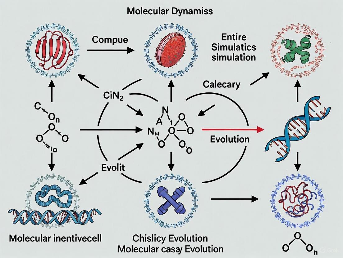
Diagram 1: Integrative modeling workflow for building an entire cell model. The process begins with experimental data, informs a mesoscale model, generates molecular components, and finally assembles the complete system.
Table 2: Key Research Reagent Solutions for MD Simulations
| Tool / Resource Name | Type | Primary Function | Relevance to Whole-Cell Modeling |
|---|---|---|---|
| GROMACS [2] | Software Package | A high-performance MD engine for simulating molecular systems. | Core simulation software for running large-scale simulations. |
| Martini Force Field [1] | Coarse-Grained Force Field | Represents ~4 heavy atoms with one bead, greatly accelerating simulation. | Enables feasible simulation of cellular-scale systems like JCVI-syn3A. |
| Martinize2 [1] | Software Tool | Automates the generation of Martini coarse-grained models from atomistic protein structures. | High-throughput topology generation for the entire proteome. |
| Polyply [1] | Software Tool | Generates topologies and coordinates for polymers, including chromosomal DNA, from sequence. | Constructing the large genomic DNA polymer of a cell. |
| Vermouth [1] | Software Library | A central Python library for graph-based molecular manipulation; underpins Martinize2 and Polyply. | Provides the unified framework for handling molecules in the Martini ecosystem. |
| Bentopy [1] | Software Tool (in dev) | Generates dense, random packings of biomolecules within defined volumes. | Packing the cytoplasm with proteins and metabolites at realistic concentrations. |
| MM/PBSA [5] | Computational Method | Calculates binding free energies from MD trajectories using an implicit solvent model. | Useful in drug discovery for evaluating ligand-protein interactions. |
Diagram 2: A generalized workflow for setting up and running a coarse-grained MD simulation using the Martini force field and its associated tools.
Why Whole-Cell Modeling? The Scientific Drive for a Holistic View
The quest to understand the fundamental units of life—cells—in their complete complexity represents one of the most ambitious goals in modern science. Whole-cell modeling emerges as a transformative approach that aims to comprehensively predict how cellular phenotypes emerge from genotype by representing the entire genome, the structure and concentration of every molecular species, each molecular interaction, and the extracellular environment [6]. This paradigm shift from studying isolated cellular components to modeling the cell in its entirety promises to bridge critical gaps in our understanding of biological systems, enabling unprecedented predictive capabilities in bioengineering and precision medicine [7] [8]. The driving vision is to create a computational microscope that reveals the dynamics of all cellular components with ultimate resolution, offering a holistic view of cellular function that transcends what can be observed through conventional experimental methods alone [1].
The scientific community's pursuit of whole-cell modeling is fueled by the recognition that biological functions emerge from the intricate, multi-scale interactions between cellular components [1] [9]. While traditional reductionist approaches have yielded profound insights into specific pathways and mechanisms, they inevitably fall short of capturing the system-level behaviors that characterize living systems. By integrating the collective knowledge of individual cellular processes into a unified framework, whole-cell models offer a pathway to understand how perturbations at the molecular level—such as genetic mutations, drug treatments, or environmental changes—propagate through the system to influence observable cellular phenotypes [10] [9]. This integrative approach is poised to revolutionize how we investigate, manipulate, and ultimately understand the fundamental processes of life.
The Scientific Imperative: Key Drivers for Whole-Cell Modeling
From Isolated Pathways to Integrated Cellular Function
Cellular processes are traditionally studied and modeled as separate networks with heterogeneous levels of detail, such as metabolic networks, protein-protein interaction networks, and transcription regulation networks [9]. However, these processes are neither physically nor functionally independent; the simple fact that molecular species are shared between them makes their dynamics interdependent [9]. For instance, the intracellular concentration of ATP affects and is affected by several processes simultaneously. Whole-cell modeling addresses this interconnected nature of cellular systems by integrating these disparate processes into a unified representation, enabling researchers to study emergent properties that arise from their interactions [9].
The limitations of studying cellular components in isolation become particularly evident when considering that biomolecular functions emerge from molecular interactions within complex, crowded cellular environments [1]. Experimental techniques, while invaluable, often probe only narrow windows in the space-time continuum of cellular activity [10]. Whole-cell modeling addresses this limitation by providing a unified framework that integrates structural and dynamic data across multiple scales, from molecular interactions to system-level behaviors [10]. This approach allows researchers to investigate how biological macromolecules behave inside cells and navigate a spectrum of specific and non-specific interactions in the presence of various electrolytes, osmolytes, and other small molecules—questions that remain difficult to address through experiment alone [10].
Predictive Power: From Genotype to Phenotype
A primary motivation for whole-cell modeling is the ability to predict cellular phenotypes from genetic information, a fundamental challenge in modern biology [6]. By comprehensively representing the function of each characterized gene product and its interactions within the cellular network, whole-cell models can simulate how genetic variations manifest as observable traits [6]. This predictive capability has profound implications for understanding disease mechanisms, developing therapeutic interventions, and engineering microorganisms for biotechnology applications.
The power of whole-cell models to connect genotype to phenotype extends beyond academic interest to practical applications in drug discovery and personalized medicine. For example, with a comprehensive whole-cell model of a bacterial pathogen like Methicillin-resistant Staphylococcus aureus (MRSA), researchers could use computer simulations informed by biological experiments to engineer new prevention and treatment strategies for antibiotic-resistant infections [8]. Similarly, in cancer treatment, a complete cell model of immune cells could enable the fine-tuning of specific anti-tumor responses to improve immunotherapies without invasive exploration of the patient [8]. These applications highlight the transformative potential of whole-cell models in translating basic biological knowledge into clinical and biotechnological advances.
Table 1: Key Application Areas of Whole-Cell Modeling
| Application Area | Specific Use Cases | Potential Impact |
|---|---|---|
| Drug Discovery & Development | Target identification, mechanism of action studies, toxicity prediction | Reduced development costs, personalized treatment approaches |
| Infectious Disease Research | Modeling of bacterial pathogens (e.g., MRSA), antibiotic resistance mechanisms | Novel therapeutic strategies for drug-resistant infections |
| Cancer Research & Treatment | Cancer immunotherapy optimization, tumor cell behavior prediction | Improved personalized cancer therapies with reduced side effects |
| Industrial Biotechnology | Metabolic engineering, optimization of production strains | Enhanced bioproduction of pharmaceuticals, chemicals, and biofuels |
| Environmental Biotechnology | Biofilm control in water treatment systems | Improved water desalination and purification processes |
Addressing the Multi-Scale Challenge of Biological Systems
Cellular function operates across multiple spatial and temporal scales, from rapid molecular interactions occurring in nanoseconds to slow cellular processes like division that take hours [10] [11]. This multi-scale nature of biological systems presents a fundamental challenge that whole-cell modeling directly addresses by integrating representations across these scales. Where traditional experimental methods struggle to simultaneously capture atomistic detail and cellular context, whole-cell models can incorporate data from diverse sources—including structural biology, omics technologies, and biophysical measurements—into a coherent computational framework [1] [10].
The multi-scale challenge extends beyond temporal considerations to encompass organizational complexity, from individual molecules to macromolecular complexes, organelles, and ultimately the entire cell [11]. Physical whole-cell models that build up from atomic-level structures of individual molecules to system-level representations offer the potential to connect behavior at the molecular level to cellular function through physical laws [10]. This approach provides a more fundamental basis for prediction compared to purely statistical or kinetic models, as it can potentially forecast how specific molecular interventions—such as drug candidates—perturb cellular function without requiring pre-existing assumptions about altered kinetic pathways [10].
Quantitative Landscape: Current Capabilities and Computational Requirements
Model Organisms and Their Complexity
Current whole-cell modeling efforts have focused on relatively simple organisms with minimal genetic complexity, enabling proof-of-concept demonstrations while laying the groundwork for more ambitious applications. The bacterium Mycoplasma genitalium, with its compact genome of approximately 500 genes, served as the first comprehensive whole-cell modeling target, integrating 15 cellular processes into a single modeling framework [9]. This pioneering work demonstrated the feasibility of whole-cell modeling and established methodologies for model construction and validation.
More recently, the minimal synthetic cell JCVI-syn3A, containing only 493 genes, has emerged as a promising model system for whole-cell simulation approaches [1]. With a diameter of approximately 400 nm and a largely resolved molecular composition, JCVI-syn3A represents an ideal testbed for developing and refining whole-cell modeling methodologies, particularly those requiring comprehensive structural and compositional data [1]. The relative simplicity of this system makes it particularly amenable to detailed computational modeling approaches that would be infeasible with more complex organisms.
Table 2: Model Organisms in Whole-Cell Modeling Studies
| Organism | Genome Size (Genes) | Key Features | Modeling Achievements |
|---|---|---|---|
| Mycoplasma genitalium | ~500 | Smallest known genome of any free-living organism | First whole-cell computational model integrating 15 cellular processes [9] |
| JCVI-syn3A | 493 | Synthetic minimal cell with reduced genetic complexity | Atomistic and coarse-grained molecular dynamics simulations [1] |
| Escherichia coli | ~4,300 | Well-studied model bacterium with extensive experimental data | Initial whole-cell modeling efforts; kinetic models of metabolism [12] |
Computational Requirements and Scaling Challenges
The computational demands of whole-cell modeling vary dramatically depending on the chosen resolution and simulation approach. Atomistic models, which provide the highest level of detail, require simulating enormous numbers of particles—a bacterial cytoplasm model may reach 100 million particles for just 1/10th to 1/20th of the smallest bacterial cell [10]. For complete cells like JCVI-syn3A, coarse-grained molecular dynamics simulations using the Martini force field require approximately 550 million coarse-grained particles, corresponding to more than six billion atoms [1].
The computational cost of these simulations presents significant challenges. State-of-the-art supercomputers like Fugaku can achieve approximately 8.3 nanoseconds per day for a 1.6 billion-atom system [11]. Specialized molecular dynamics supercomputers like Anton 3 offer improved performance, with a 512-node machine capable of simulating timescales of milliseconds per day for systems approximating a eukaryotic cell (∼100 trillion atoms) [11]. These computational constraints have driven the development of multi-resolution approaches that combine different levels of molecular detail, applying atomistic resolution only to specific regions of interest while treating the remaining cellular environment with more efficient coarse-grained methods [10] [11].
Methodological Approaches: Experimental Protocols in Whole-Cell Modeling
Integrative Modeling Workflow for Whole-Cell Model Construction
The construction of whole-cell models follows an integrative workflow that synthesizes diverse experimental data into coherent computational representations. This process typically begins with the collection of experimental data from multiple sources, including cryo-electron tomography (cryo-ET) images, cryo-EM protein structures, and various -omics experiments (genomics, proteomics, metabolomics) [1]. These data provide essential information about cellular architecture, molecular structures, and composition that informs the subsequent modeling stages.
The second stage involves mesoscale modeling, where kinetic models of cellular processes are developed to gain quantitative insights into cellular processes and composition [1]. These models often employ constraint-based methods, ordinary differential equations, or rule-based approaches to capture the dynamics of metabolic networks, gene expression, and other essential cellular functions. In the final stage, molecular-resolution models of cellular components are generated using specialized software tools, followed by the assembly of individual molecular components in their appropriate abundances into the final whole-cell model [1]. This multi-stage approach allows for the integration of data across spatial and temporal scales, bridging from molecular structure to cellular function.
Diagram 1: Integrative modeling workflow for building in silico whole-cell models, illustrating the three major stages from data collection to final model assembly.
Protocol: Building a Coarse-Grained Whole-Cell Model with the Martini Ecosystem
The Martini coarse-grained force field has emerged as a powerful tool for whole-cell modeling, offering a balance between computational efficiency and molecular detail. The following protocol outlines the key steps for constructing a coarse-grained whole-cell model using the Martini ecosystem:
Step 1: System Preparation and Component Selection
- Select the target organism (e.g., JCVI-syn3A minimal cell) and gather comprehensive compositional data
- Obtain or generate structural models for all macromolecular components (proteins, DNA, RNA)
- Determine the stoichiometry and cellular abundances of all molecular species from experimental data [1]
Step 2: Topology Generation for Cellular Components
- For proteins: Use Martinize2 software to generate Martini topologies and coordinates from atomistic protein structures [1]. This tool performs quality checks on atomistic structures and alerts to potential problems.
- For chromosomal DNA: Employ Polyply software to efficiently generate polymer topologies from sequence data using a multiresolution graph-based approach [1]
- For lipids: Use the Martini Database to access curated parameters for various lipid species [1]
- For metabolites: Apply recently developed Martini parameters for small molecules [1]
Step 3: System Assembly
- Use specialized packing software like Bentopy (currently in development) to generate dense macromolecular solutions within volumetric constraints that reflect cellular crowding [1]
- Incorporate functional annotations to bias spatial distribution of proteins based on known biochemical functions
- Assemble membrane systems using insane tool or similar utilities for building complex membrane architectures [1]
Step 4: Simulation Setup and Execution
- Integrate the assembled system using simulation packages like GROMACS capable of handling large-scale systems
- Implement appropriate simulation parameters accounting for the Martini force field requirements
- Run simulations on high-performance computing resources, potentially leveraging GPU acceleration for improved performance
Step 5: Analysis and Validation
- Compare simulation results with experimental data for validation
- Analyze spatial organization, diffusion characteristics, and emergent behaviors
- Iteratively refine the model based on discrepancies between simulation and experiment
This protocol leverages the growing Martini ecosystem of software tools specifically designed to facilitate the construction of topologies and initial coordinates for running coarse-grained molecular dynamics simulations of complex cellular systems [1].
Protocol: Biochemical Network Modeling for Whole-Cell Integration
An alternative approach to whole-cell modeling involves constructing comprehensive biochemical networks that integrate multiple cellular processes. The following protocol outlines the key steps for this methodology:
Step 1: Data Integration and Curation
- Collect organism-specific biochemical data from databases such as WholeCellKB, MetaCyc, BRENDA, and UniProt [9] [6]
- Map known molecular interactions, including metabolic reactions, protein-protein interactions, and transcriptional regulation relationships
- Resolve inconsistencies and gaps in the data through manual curation and literature review
Step 2: Rule-Based Model Specification
- Define reaction rules that can be applied to multiple substrates following rule-based modeling principles [9]
- Develop templates for repetitive processes such as transcription, translation, and replication that can be instantiated for specific genes or macromolecules [9]
- Specify modification rules for post-translational modifications and other chemical alterations
Step 3: Network Generation
- Instantiate the rule set to generate specific biochemical reactions for all molecular components
- Represent the system as a bipartite graph with molecule nodes and reaction nodes connected by edges indicating participation as reactants, products, or modifiers [9]
- Annotate edges with stoichiometric information and regulatory effects
Step 4: Model Validation through Essentiality Prediction
- Implement cascading failure analysis to simulate gene deletions [9]
- Compare predicted essential genes with experimental data from global transposon mutagenesis studies [9]
- Refine the model to improve agreement between predictions and experimental observations
Step 5: Simulation and Analysis
- Employ constraint-based methods such as flux balance analysis to simulate metabolic behavior [12]
- Implement kinetic simulations for dynamic processes where parameter data are available
- Analyze network properties to identify critical nodes, bottlenecks, and functional modules
This biochemical network approach provides a more homogeneous framework for whole-cell modeling compared to hybrid approaches that combine multiple modeling methodologies [9]. It enables a systemic analysis of cells on a broader scale, revealing interfaces between cellular processes that might be obscured in more segregated modeling frameworks.
Table 3: Research Reagent Solutions for Whole-Cell Modeling
| Resource Category | Specific Tools/Databases | Function/Purpose |
|---|---|---|
| Structural Biology Databases | Protein Data Bank (PDB), Cryo-EM Data Bank, AlphaFold Protein Structure Database | Provide atomic-level structural information for proteins and nucleic acids essential for physical modeling [10] [11] |
| Omics Data Resources | WholeCellKB, PaxDb, ECMDB, ArrayExpress | Offer comprehensive datasets on cellular composition, including protein abundances, metabolite concentrations, and gene expression profiles [12] [9] [6] |
| Pathway/Interaction Databases | KEGG, MetaCyc, BioCyc, BRENDA, SABIO-RK | Contain curated information about metabolic pathways, regulatory networks, and kinetic parameters [12] [6] |
| Modeling Software & Platforms | Martini Ecosystem (Martinize2, Polyply, Vermouth), E-CELL, Virtual Cell, COPASI, PySB | Provide specialized tools for constructing, simulating, and analyzing whole-cell models at different resolutions [1] [12] [6] |
| Simulation Force Fields | Martini Coarse-Grained Force Field, All-Atom Force Fields (CHARMM, AMBER) | Define interaction parameters between molecular components at different resolutions [1] [10] |
| Standards & Formats | Systems Biology Markup Language (SBML), CellML | Enable model sharing, reproducibility, and interoperability between different modeling tools [12] |
Future Directions: Integrating Artificial Intelligence and Advanced Computing
The future of whole-cell modeling is increasingly intertwined with advances in artificial intelligence (AI) and machine learning (ML). These technologies are poised to address two critical challenges in molecular simulations: force field accuracy and sampling efficiency [11]. Neural networks for predicting force field parameters have been shown to approach the accuracy of traditional quantum mechanics-based methods while being approximately three orders of magnitude more efficient [11]. Similarly, enhanced sampling methods like reinforced dynamics protocols enable more efficient exploration of complex energy landscapes, making it feasible to simulate cellular processes at relevant timescales [11].
The integration of AI methods with structural biology breakthroughs is creating new opportunities for whole-cell modeling. The availability of predicted three-dimensional models for entire proteomes through AlphaFold, combined with high-resolution structural data from cryo-electron microscopy, is rapidly filling the gaps in our structural knowledge of cellular components [11] [13]. Meanwhile, cryo-electron tomography provides unprecedented insights into cellular architecture in situ, informing more realistic model assemblies [1] [11]. These advances, coupled with the exponential growth in computational power and the emergence of MD simulation-specific supercomputers, suggest that comprehensive physical simulations of entire cells may be achievable in the foreseeable future [11].
Diagram 2: Future directions in whole-cell modeling showing the integration of artificial intelligence, structural biology advances, and advanced computing hardware.
Whole-cell modeling represents a paradigm shift in computational biology, offering a pathway to understand cellular behavior through integrated, multi-scale representations rather than isolated components. The scientific drive for this holistic view stems from the recognition that cellular functions emerge from the complex interactions between countless molecular components, and that a comprehensive understanding requires models that capture this complexity [7] [9]. While significant challenges remain in model construction, validation, and simulation, the rapid advances in experimental methods, computational power, and algorithmic approaches are quickly making whole-cell modeling a viable approach for tackling fundamental questions in biology [10] [11].
The potential applications of whole-cell models span from basic science to translational research, including drug discovery, personalized medicine, biotechnology, and beyond [8] [6]. As these models continue to develop and improve, they promise to transform how we investigate cellular processes, design therapeutic interventions, and engineer biological systems. By providing a computational framework that integrates our collective knowledge of cellular components and their interactions, whole-cell modeling offers the tantalizing possibility of predicting cellular behavior from first principles—a capability that would fundamentally advance our understanding of life and our ability to manipulate it for human benefit.
JCVI-syn3A represents a landmark achievement in synthetic biology and a transformative platform for computational modeling. This minimal cell, derived from Mycoplasma mycoides, contains a synthetically designed genome of only 543 kilobase pairs with 493 genes, making it the smallest genome of any known self-replicating organism [14] [15] [16]. Its drastically reduced complexity compared to natural bacterial cells—approximately one-tenth the genomic size of E. coli—makes it an ideal benchmark for developing and validating whole-cell computational models [17] [18]. The creation of JCVI-syn3A was driven by the fundamental question of what constitutes the minimal genetic requirements for life, providing a streamlined biological system where cellular processes can be studied without the redundancy and complexity of natural organisms [16] [19].
This minimal cell platform has emerged as a powerful testbed for computational biologists aiming to build predictive models of entire cells. Unlike traditional models that focus on isolated cellular pathways, JCVI-syn3A enables researchers to simulate integrated cellular functions from metabolism to replication within a manageable parameter space [17] [18]. With 92 genes still of unknown function in JCVI-syn3A, computational models serve not only as validation tools but also as hypothesis generators for discovering new biological mechanisms essential for life [18]. The integration of multi-scale data from genomics, proteomics, structural biology, and cryo-electron microscopy has positioned JCVI-syn3A at the forefront of efforts to simulate complete cellular systems using molecular dynamics and other computational approaches [14] [20] [21].
Genomic and Structural Characteristics
JCVI-syn3A exhibits distinctive structural and genomic properties that make it uniquely suited for whole-cell modeling. The cell measures approximately 400 nm in diameter, significantly smaller than most natural bacteria [14]. Its genome was systematically minimized through design-build-test cycles, starting from JCVI-syn1.0 (with 901 genes) and progressively removing non-essential genetic elements while maintaining capacity for autonomous replication [15] [16]. This minimization process identified both essential genes (immediately required for survival) and quasi-essential genes (necessary for robust growth but dispensable under ideal conditions) [15].
The structural organization of JCVI-syn3A, while simplified, maintains the fundamental compartments of a prokaryotic cell. The cell envelope consists of a lipid membrane without a cell wall, characteristic of Mycoplasma species [19]. Internal organization includes a nucleoid region containing the circular chromosome, ribosomes for protein synthesis, and various metabolic enzymes dispersed throughout the cytosol [20] [21]. The minimal genome has forced a high efficiency in molecular organization, with approximately 40% of the intracellular volume occupied by proteins [14]. This dense packing creates a highly crowded intracellular environment that influences molecular diffusion and interaction kinetics—a critical consideration for accurate physical modeling [14].
Table 1: Key Characteristics of JCVI-syn3A Minimal Cell
| Parameter | Specification | Significance for Modeling |
|---|---|---|
| Genome Size | 543 kbp | Drastically reduced sequence space for simulation |
| Number of Genes | 493 total (452 protein-coding) | Manageable number of molecular components |
| Genes of Unknown Function | 92 (20% of protein-coding genes) | Opportunity for discovery via model prediction |
| Physical Diameter | ~400 nm | Computationally tractable for 3D simulation |
| Doubling Time | 105-120 minutes | Definable cell cycle for temporal models |
| Chromosome Topology | Single circular DNA molecule | Simplified genome organization |
Metabolic Capabilities and Essential Functions
Despite its minimal genome, JCVI-syn3A maintains a surprisingly comprehensive metabolic network capable of synthesizing most essential biomolecules. The reconstructed metabolic network accounts for 98% of enzymatic reactions supported by experimental evidence or annotation [15]. Key metabolic pathways include central carbon metabolism, nucleotide biosynthesis, amino acid metabolism, and lipid biosynthesis, though the cell relies on scavenging some nutrients from its environment [15]. The model organism requires specifically enriched culture medium containing metabolic precursors that it cannot synthesize independently, reflecting the trade-offs made during genome minimization [15] [18].
The essential functions encoded by the minimal genome can be categorized into several core cellular processes: genetic information processing (DNA replication, transcription, translation), energy production, membrane biogenesis, and cellular division [18]. Analysis of gene essentiality shows that 68% of genes are strictly essential for survival, with an additional 24% classified as quasi-essential, bringing the total essentiality to 92% [15]. This high essentiality fraction underscores the efficiency of the minimized genome, with most genes serving non-redundant critical functions. The metabolic model agrees well with genome-scale in vivo transposon mutagenesis experiments, showing a Matthews correlation coefficient of 0.59 [15], validating its accuracy for predictive simulations.
Computational Modeling Approaches
Molecular Dynamics Frameworks
Molecular dynamics (MD) simulations of JCVI-syn3A leverage coarse-grained approaches to manage the enormous computational challenge of simulating an entire cell. The Martini force field has emerged as the primary framework for these simulations, employing a four-to-one mapping scheme where up to four heavy atoms and associated hydrogens are represented by a single coarse-grained bead [14]. This reduction decreases the number of particles in the system by approximately fourfold, speeding up simulations by about three orders of magnitude while maintaining sufficient chemical specificity [14]. For JCVI-syn3A, this approach requires about 550 million coarse-grained particles, corresponding to more than six billion atoms—a scale that would be computationally prohibitive with all-atom models [14].
The Martini ecosystem provides specialized tools for each cellular component. Martinize2 generates topologies and coordinates for proteins from atomistic structures [14]. Polyply handles nucleic acids, using a multiresolution graph-based approach to efficiently generate polymer topologies from sequence data [14]. TS2CG converts triangulated surfaces into coarse-grained membrane models, enabling simulation of the cell envelope with precise control over lipid composition and curvature [14]. These tools collectively enable construction of a comprehensive whole-cell model that integrates proteins, nucleic acids, lipids, and metabolites within a unified simulation framework.
Integrative Modeling of Cellular Structures
Integrative modeling approaches combine cryo-electron tomography data with genomic and proteomic information to create accurate 3D structural models of JCVI-syn3A components. For the nucleoid, lattice-based methods generate initial models with one bead per ten base pairs, incorporating user-defined superhelical plectonemes and coarse-grain representations of nucleoid-associated proteins [20] [22]. These models are then optimized off-lattice with constraints for connectivity, steric occlusion, and fiber stiffness [20]. The resulting structures faithfully represent the genome organization while remaining computationally tractable for simulation.
The modular modeling pipeline implements "molecular masks" for key nucleoid-related complexes including RNA polymerase, ribosomes, and structural maintenance of chromosomes (SMC) cohesins [20]. These masks are positioned based on cryo-electron tomography data, with ribosomes placed at experimentally determined positions and other components distributed according to biochemical constraints [20]. The models successfully integrate ultrastructural information with molecular-level detail, enabling hypothesis testing about transcription, genome condensation, and spatial organization of genetic material [20].
Diagram: Integrative modeling workflow for JCVI-syn3A, showing the pipeline from experimental data to model predictions.
Application Notes: Simulation Protocols
Whole-Cell Model Construction Protocol
Objective: Construct a computationally tractable coarse-grained model of an entire JCVI-syn3A cell for molecular dynamics simulation.
Materials and Software Requirements:
- Martini ecosystem tools (Vermouth, Martinize2, Polyply, TS2CG)
- Genomic sequence of JCVI-syn3A (GenBank accessions)
- Proteomic and lipidomic composition data
- Cryo-electron tomography structural data
- High-performance computing infrastructure
Procedure:
- Genome Structure Generation
- Input circular chromosome sequence (543 kbp) into Polyply software
- Generate double-stranded DNA model with 10 bp/bead resolution
- Introduce superhelical density of -0.06 to form physiological plectonemes
- Set persistence length to 50 nm for DNA mechanical properties
Proteome Integration
- Obtain atomic structures for all 452 JCVI-syn3A proteins from PDB or homology modeling
- Process each protein through Martinize2 for Martini coarse-graining
- Use Bentopy for efficient collision detection and packing of proteins within cytoplasmic volume constraints
- Incorporate functional annotations to bias spatial distribution based on biological function
Membrane Assembly
- Define membrane curvature based on cryo-ET measurements of cell morphology
- Input lipid composition (phospholipids, glycolipids) from mass spectrometry data
- Generate membrane model using TS2CG with triangulated surface representation
- Insert transmembrane proteins with characteristic lipid shells using lipid fingerprint data
System Integration and Equilibration
- Combine all components in simulation box with appropriate ionic conditions
- Perform energy minimization using steepest descent algorithm
- Conduct stepwise equilibration with position restraints gradually released
- Run production molecular dynamics simulation using GROMACS with Martini parameters
Validation Metrics:
- Compare simulated cell diameter to experimental measurements (~400 nm)
- Verify reproduction of experimental doubling time (105-120 minutes)
- Confirm appropriate density of cytoplasmic proteins (~40% volume fraction)
- Validate structural stability over multiple replication cycles
Nucleoid Modeling Protocol
Objective: Generate a 3D structural model of the JCVI-syn3A nucleoid integrating experimental data and molecular details.
Materials and Software Requirements:
- ModularLattice software package
- Cryo-ET segmented ribosome positions
- Genomic sequence with gene annotations
- Structures of RNA polymerase, ribosomes, SMC complexes
Procedure:
- Molecular Mask Preparation
- Generate lattice-based models of RNA polymerase (PDB 6c6u), ribosomes (PDB 4v6k), and SMC cohesins (PDB 7nyx)
- Embed each molecular structure in a 3.4 nm grid, selecting points within one grid spacing of atoms
- Manually assign control points for DNA/RNA/protein chain connections
- Add insulating points around control points to prevent occlusion
Component Placement
- Import experimentally determined ribosome positions (503 total)
- Place ribosome masks with random orientations from 24 possible 90° rotations
- Resolve minor clashes through local jittering of positions
- Place RNA polymerases (187 total) via random walk algorithm in free spaces
- Position SMC complexes (187 total) between polymerase locations
Genome Tracing and Connectivity
- Connect molecular masks with DNA segments using biased random walk
- Implement user-defined supercoiling for DNA segments
- Connect RNA polymerases to ribosomes via mRNA chains
- Ensure single circular DNA continuity throughout nucleoid
Structural Refinement
- Optimize model off-lattice with connectivity constraints
- Apply steric exclusion constraints between all components
- Enforce appropriate fiber stiffness for DNA and RNA chains
- Perform Monte Carlo relaxation to eliminate residual clashes
Validation:
- Verify genome occupies appropriate nucleoid volume fraction
- Confirm compatibility with Hi-C contact probability data
- Check appropriate spatial segregation of transcription and translation
- Validate mechanical properties against single-molecule experiments
Table 2: Key Quantitative Parameters for JCVI-syn3A Simulations
| Simulation Parameter | Value | Computational Impact |
|---|---|---|
| Coarse-Grained Particles | ~550 million | Enables millisecond timescales on exascale computing |
| Simulation Box Size | ~500 nm³ | Requires massive parallelization across GPU clusters |
| Temporal Resolution | 20-50 fs | Balances numerical stability with simulation speed |
| Simulation Duration | 1-10 μs | Captures complete cell division cycles |
| Energy Calculations | ~2000 reactions | Tracks metabolic flux and energy budgets |
Research Reagent Solutions
The computational study of JCVI-syn3A relies on both in silico tools and physical research reagents that enable model validation. The table below details essential resources for JCVI-syn3A research.
Table 3: Essential Research Reagents and Computational Tools for JCVI-syn3A Studies
| Resource Name | Type | Function | Access Information |
|---|---|---|---|
| Martini Force Field | Computational Tool | Coarse-grained molecular dynamics parameters | Martini Database (https://mdmartini.nl) |
| Polyply | Software | Graph-based generation of nucleic acid structures | GitHub Repository (https://github.com/marrink-lab/polyply) |
| JCVI-syn3A Genome | Biological Data | Minimal genome sequence | GenBank CP014940.1 |
| ModularLattice | Software | Lattice-based nucleoid modeling | GitHub (https://github.com/ccsb-scripps/ModularNucleoid) |
| Cryo-ET Tomograms | Experimental Data | Cellular ultrastructure reference | Available upon collaboration |
| Metabolic Network Model | Computational Model | Constraint-based metabolic flux analysis | Supplementary materials from [15] |
Signaling and Metabolic Pathways
JCVI-syn3A contains streamlined versions of essential metabolic pathways that represent core energy production and biosynthetic capabilities. The major metabolic routes include glycolysis, pentose phosphate pathway, nucleotide biosynthesis, and limited amino acid metabolism [15] [18]. The metabolic model successfully predicts flux distributions that match experimental measurements of nutrient consumption and growth rates, providing validation of its accuracy [15].
A key feature of JCVI-syn3A's metabolism is its heavy reliance on substrate-level phosphorylation for energy generation rather than oxidative phosphorylation [15]. This simplification reflects the minimal genome's elimination of many electron transport chain components, resulting in exclusively fermentative metabolism. The model predicts and experiments confirm that addition of specific non-essential genes can enhance metabolic efficiency, such as the 13% reduction in doubling time observed when pyruvate dehydrogenase genes were added back to the minimal genome [18].
Diagram: Core metabolic network of JCVI-syn3A showing simplified metabolic pathways and their connections to cellular functions.
JCVI-syn3A has established a new benchmark for whole-cell modeling, demonstrating that predictive simulation of an entire living organism is computationally achievable when biological complexity is sufficiently minimized. The integration of multi-scale data from cryo-electron tomography, proteomics, and metabolomics with molecular dynamics frameworks has produced models that accurately recapitulate observed cellular behaviors, including growth rates and structural organization [14] [18]. These models serve not only as validation tools but as discovery platforms, generating testable hypotheses about the function of uncharacterized essential genes and enabling in silico experiments that would be resource-intensive to perform in the laboratory [17] [18].
Future developments in JCVI-syn3A modeling will focus on increasing spatial and temporal resolution while expanding the scope of cellular processes represented. Current efforts aim to integrate stochastic gene expression with metabolic flux models to predict phenotypic variability in clonal populations [18]. As computational power increases through exascale computing, all-atom simulations of subcellular compartments may become feasible, providing atomic-level insights into molecular mechanisms within the context of the full cellular environment [14]. The JCVI-syn3A platform continues to evolve as a testbed for developing computational methods that will eventually be applied to more complex model organisms and human cells, advancing toward the ultimate goal of predictive whole-cell modeling for biomedical and biotechnological applications [17].
Spatial Resolution, Timescales, and the 'Computational Microscope'
Molecular dynamics (MD) simulation has matured into a powerful tool that functions as a computational microscope, enabling researchers to probe biomolecular processes at an atomic level of detail that is often difficult or impossible to achieve with experimental techniques alone [14] [23]. This "microscope" provides an exceptional spatio-temporal resolution, revealing the dynamics of cellular components and their interactions [24]. The application of this technology to model an entire cell represents a monumental step forward in computational biology, offering the potential to interrogate a cell's spatio-temporal evolution in unprecedented detail [14] [1]. This article details the key concepts, quantitative parameters, and experimental protocols for employing MD simulations to study biological systems at the scale of a complete minimal cell.
Key Quantitative Parameters
The utility of the computational microscope is defined by its ability to resolve specific spatial and temporal characteristics. The following parameters are critical for planning and interpreting simulations, especially for large-scale systems like an entire cell.
Table 1: Key Spatio-Temporal Parameters in Molecular Dynamics Simulations
| Parameter | Typical Range | Description | Biological Relevance |
|---|---|---|---|
| Spatial Resolution | Atomic (Ã…) to Coarse-Grained (nm) | Level of structural detail captured. | From atomic interactions (all-atom) to macromolecular assembly dynamics (coarse-grained). |
| Temporal Resolution | 0.5 - 2.0 femtoseconds (fs) | Time interval between simulation steps [25]. | Determines the fastest motions that can be accurately captured (e.g., bond vibrations). |
| Total Simulation Time | Nanoseconds (ns) to Milliseconds (ms) | Total physical time covered by the simulation [24]. | Determines which biological processes can be observed (e.g., local dynamics vs. protein folding). |
| System Size (All-Atom) | Millions to Billions of atoms | Number of atoms in the simulation box. | From single proteins to sub-cellular structures or minimal cells (e.g., ~6 billion atoms for JCVI-syn3A) [14]. |
| System Size (Coarse-Grained) | Hundreds of Millions of particles | Reduced number of interaction sites, speeding up calculations. | Enables simulation of mesoscale systems like entire cells (e.g., ~550 million particles for JCVI-syn3A) [14]. |
Workflow for Whole-Cell Modeling and Simulation
Constructing and simulating an entire cell requires an integrative modeling approach that synthesizes diverse experimental data into a coherent computational framework [14] [1]. The workflow involves multiple stages, from data collection to final analysis.
Diagram Title: Integrative Workflow for Whole-Cell MD Simulation
The Martini Ecosystem: A Toolkit for Mesoscale Simulation
For modeling systems as vast as an entire cell, a coarse-grained (CG) approach is indispensable. The Martini force field is a leading CG model that employs a four-to-one mapping scheme, where up to four heavy atoms are represented by a single CG bead [14]. This reduction, combined with a smoothened potential energy surface, accelerates simulations by approximately three orders of magnitude, making cellular-scale modeling feasible [14]. The Martini "ecosystem" comprises a suite of software tools designed to work together.
Table 2: Essential Research Reagent Solutions for Whole-Cell MD
| Tool / Resource | Type | Primary Function | Application in Whole-Cell MD |
|---|---|---|---|
| Martini Force Field | Coarse-Grained Force Field | Defines interaction parameters for biomolecules [14]. | Provides the physical model for efficient simulation of large, complex cellular systems. |
| Martinize2 | Software Tool | High-throughput generation of Martini topologies for proteins [14]. | Automates the conversion of the proteome (hundreds of proteins) into CG representations. |
| Polyply | Software Tool | Generates topologies and coordinates for polymeric systems like DNA [14]. | Constructs large chromosomal DNA structures from sequence data. |
| Bentopy | Software Tool (In Dev) | Efficiently packs proteins and complexes into dense solutions [14]. | Assembles the crowded cytoplasmic environment based on functional annotations and abundances. |
| TS2CG | Software Tool | Converts triangulated surfaces into CG membrane models [14]. | Builds complex cell envelopes with curvature-dependent lipid composition. |
| Vermouth | Python Library | Graph-based framework unifying Martini processes [14]. | Serves as the central, interoperable foundation for many ecosystem tools. |
| GROMACS | MD Simulation Engine | High-performance software to run MD simulations [26]. | Executes the production MD simulation, often optimized for GPUs. |
| Calcium plumbate | Calcium Plumbate Supplier | 12013-69-3 | For Research | High-purity Calcium Plumbate (Ca2O4Pb) for materials science and corrosion research. For Research Use Only. Not for human or veterinary use. | Bench Chemicals |
| FMePPEP | FMePPEP, CAS:1059188-86-1, MF:C26H24F4N2O2, MW:472.47 | Chemical Reagent | Bench Chemicals |
Application Note: Modeling the JCVI-syn3A Minimal Cell
Background and Rationale
The minimal cell JCVI-syn3A (Syn3A), created by the J. Craig Venter Institute, is an ideal candidate for whole-cell modeling [14] [1]. With a diameter of only 400 nm and a stripped-down genome of 493 genes, its relative simplicity makes the immense challenge of a full-cell simulation tractable [14]. Its composition has been extensively characterized, providing the necessary quantitative data for integrative modeling [1].
Detailed Protocol for Constructing the Syn3A Model
Step 1: Chromosome Building
- Input: The circular chromosome sequence of 543 kbp.
- Tool: Polyply.
- Method: Use the graph-based and biased random walk protocols within Polyply to generate the three-dimensional structure and Martini topology of the chromosomal DNA directly from its sequence. This avoids the computational intractability of forward-mapping from an all-atom structure [14].
- Output: A coarse-grained model of the entire circular chromosome.
Step 2: Cytoplasmic Packing
- Input: The proteome of Syn3A, including the identity, structure, and abundance of all proteins.
- Tool: Martinize2 for protein topology generation; Bentopy for spatial packing.
- Method:
- Process all protein structures through Martinize2 to generate their CG representations.
- Use Bentopy to perform collision-detection-based packing of all cytoplasmic components, including proteins, ribosomes, and metabolites, into the defined cytosolic volume. The packing can be biased using functional annotations to create a biologically realistic distribution [14].
- Output: A densely packed, crowded cytoplasm model.
Step 3: Cell Envelope Assembly
- Input: Lipid composition data for the cell membrane.
- Tool: TS2CG.
- Method:
- Define a triangulated surface representing the cell membrane.
- Use TS2CG's backmapping algorithm to populate the membrane with lipids according to the specified composition. The tool allows precise control over the lipid distribution in both membrane leaflets [14].
- Insert membrane proteins with their characteristic lipid shells (lipid fingerprints).
- Output: A complete, protein-studded model of the cell membrane.
Step 4: System Integration and Simulation
- Input: The assembled components (chromosome, cytoplasm, membrane).
- Tool: A molecular dynamics engine like GROMACS.
- Method:
- Combine all components into a single simulation system.
- Solvate the system with the appropriate CG water model.
- Add ions to neutralize the system and achieve physiological salt concentration.
- Energy-minimize the system to remove steric clashes.
- Equilibrate the system with positional restraints on non-solvent components, then gradually release restraints.
- Run the production simulation. For Syn3A, this involves propagating ~550 million CG particles, a task requiring massive parallelization on high-performance computing (HPC) systems, often leveraging GPUs [14].
Visualization of the Martini Ecosystem
The following diagram illustrates how the various tools in the Martini ecosystem interact to build a complete cell model.
Diagram Title: Software Architecture of the Martini Ecosystem
Analysis of Simulation Trajectories
The raw output of an MD simulation is a trajectory file containing the time-evolving coordinates of all particles. Extracting scientific insight requires sophisticated analysis.
Essential Analysis Techniques
- Root Mean Square Fluctuation (RMSF): Measures the deviation of a particle (e.g., a protein's Cα atom) from its average position, quantifying flexibility and thermal fluctuations [27].
- Principal Component Analysis (PCA): Identifies the dominant collective motions (essential dynamics) in a system by diagonalizing the covariance matrix of atomic displacements. This reduces the high-dimensional trajectory data to a few key modes that often correlate with biological function [25].
- Radial Distribution Function (RDF): Quantifies the short-range order in a system, such as the solvation shell around an ion or the packing of molecules in the cytoplasm [25].
- Mean Square Displacement (MSD) & Diffusion Coefficient: The MSD measures the average squared distance a particle travels over time. In the diffusive regime, the slope of the MSD vs. time plot is used to calculate the diffusion coefficient (D), providing a quantitative measure of molecular mobility within the crowded cellular environment [25].
Statistical Significance in MD
A critical consideration when analyzing MD trajectories is the sampling problem. Due to the high dimensionality of conformational space, independent simulations started from slightly different conditions can yield different results [28] [27]. Therefore, it is essential to perform multiple replicate simulations and employ statistical tests (e.g., t-tests, Kolmogorov-Smirnov tests) to determine whether observed differences (e.g., between wild-type and mutant proteins) are statistically significant and not merely artifacts of incomplete sampling [28] [27].
The ambitious goal of building a virtual cell—a computational model capable of accurately simulating cellular behaviors in silico—represents a frontier in computational biology with the potential to revolutionize biomedical research and drug discovery [29]. Current state-of-the-art cellular simulations operate across multiple spatial and temporal scales, employing diverse computational strategies. These range from molecular dynamics (MD) simulations that model cellular components at near-atomic resolution to generative AI models that predict morphological changes in response to perturbations, and agent-based models that simulate multi-cellular systems [29] [1] [30]. Driving these advances are increases in computational power, the development of sophisticated machine learning algorithms, and the generation of massive, high-quality datasets through automated high-content screening [29] [31]. This article details the key methodologies, applications, and protocols underpinning the latest breakthroughs in cellular simulation, framed within the context of a broader thesis on molecular dynamics simulation of entire cells.
State-of-the-Art Simulation Paradigms
Whole-Cell Molecular Dynamics at Coarse-Grained Resolution
Objective: To construct a dynamic, molecular-scale model of an entire cell, capturing the spatio-temporal interactions of all its components.
Rationale: While traditional MD simulations provide unparalleled detail, their computational cost has historically limited their application to cellular subsystems. The use of coarse-grained (CG) force fields like Martini, which reduces system complexity by representing groups of atoms as single interaction beads, has enabled a leap in simulation scale [1] [14]. This approach has been successfully applied to create integrative models of a minimal cell, JCVI-syn3A, which contains only 493 genes and is one of the simplest self-replicating organisms known [1] [14].
- Proof of Concept: A proof-of-concept model of the JCVI-syn3A cell requires approximately 550 million CG particles, corresponding to more than six billion atoms, showcasing the immense scale now achievable [14].
- The Martini Ecosystem: Building and simulating an entire cell relies on a suite of integrated software tools [1] [14]:
- Vermouth: A central framework for unified handling of Martini topologies and coordinate generation.
- Martinize2: High-throughput generation of Martini topologies for proteins from atomistic structures.
- Polyply: Efficient generation of topologies and initial coordinates for large polymeric systems like chromosomal DNA.
- TS2CG: Converts triangulated surfaces into CG membrane models with precise lipid composition.
- Bentopy: Generates dense, crowded protein solutions representative of the cellular interior.
Table 1: Key Performance Metrics in State-of-the-Art Cellular Simulations
| Simulation Type | System Scale | Key Performance Metric | Reported Value / Achievement |
|---|---|---|---|
| Whole-Cell MD (Coarse-Grained) | JCVI-syn3A Minimal Cell | Number of CG Particles / Atoms Represented | ~550 million particles (>6 billion atoms) [1] [14] |
| Cellular Morphology Prediction (CellFlux) | Chemical & Genetic Perturbation Datasets (BBBC021, RxRx1, JUMP) | Fréchet Inception Distance (FID) Improvement | 35% improvement over previous methods [29] |
| Mode-of-Action Prediction Accuracy | 12% increase in accuracy [29] | ||
| Multi-Cellular Simulation (CellSys) | Tumor Spheroids & Monolayers | Maximum Simulated Cell Count | Up to several million cells [30] |
Generative AI for Predicting Cellular Morphology
Objective: To simulate how cellular morphology changes in response to chemical and genetic perturbations by learning a distribution-to-distribution mapping.
Rationale: Traditional microscopy is destructive, preventing direct observation of the same cell before and after a perturbation. CellFlux, a state-of-the-art model, overcomes this by using flow matching to learn the transformation from a distribution of unperturbed (control) cell images to a distribution of perturbed cell images [29]. This approach inherently corrects for experimental artifacts like batch effects and enables continuous interpolation between cellular states.
- Input and Output: The model takes as input an unperturbed cell image and a specified perturbation (e.g., a drug or genetic modification). It outputs a predicted image of the cell after the perturbation, faithfully capturing morphology changes specific to that intervention [29].
- Performance: Evaluated on major chemical (BBBC021), genetic (RxRx1), and combined perturbation (JUMP) datasets, CellFlux generates high-fidelity images that improve upon existing methods, as measured by a 35% improvement in FID scores and a 12% increase in mode-of-action prediction accuracy [29].
Agent-Based Modeling of Multi-Cellular Systems
Objective: To simulate growth and organization processes in multi-cellular systems, such as avascular tumor spheroids and regenerating tissues.
Rationale: Understanding tissue-level phenomena requires modeling cells as discrete, interacting agents. Software like CellSys implements an off-lattice, agent-based model where each cell is represented as an isotropic, elastic, and adhesive sphere [30].
- Biophysical Foundation: Cell migration is governed by a Langevin equation of motion, and cell-cell interactions are modeled using the experimentally validated Johnson-Kendall-Roberts (JKR) model, which summarizes deformation, compression, and adhesion forces [30].
- Applications: This methodology has been used to model liver regeneration after toxic damage, leading to predictions of cell alignment mechanisms along microvessels that were subsequently validated experimentally [30].
Application Notes & Experimental Protocols
Application Note: Simulating Perturbation Responses with CellFlux
1. Purpose To provide a protocol for using the CellFlux model to simulate the morphological changes in cells induced by a specific chemical or genetic perturbation.
2. Background CellFlux employs flow matching, a generative technique that uses an ordinary differential equation (ODE) to continuously transform the distribution of control cell images into the distribution of perturbed cell images. This allows for the in silico prediction of perturbation effects, correcting for batch artifacts and enabling the exploration of intermediate cellular states through interpolation [29].
3. Materials and Data Requirements
- Software: CellFlux codebase (publicly available).
- Data: A dataset containing paired sets of control and perturbed cell images from the same experimental batch. Standard datasets include BBBC021 (chemical), RxRx1 (genetic), or JUMP (combined).
- Input Specifications: Multi-channel microscopy images (e.g., H × W × C) from high-content screening, such as cell painting assays [29].
4. Step-by-Step Protocol
- Step 1: Data Preprocessing. Prepare and normalize the microscopy images. Ensure control and perturbed image sets are correctly assigned and batched.
- Step 2: Model Loading. Load the pre-trained CellFlux model, which includes the learned neural network approximating the velocity field for the distribution transformation.
- Step 3: Conditioning. For a given simulation, input a control cell image (
x0) and the desired perturbation condition (c). - Step 4: Sampling. Sample from the conditional distribution
p(x1|x0, c)by solving the ODE defined by the flow matching model. This generates a new, synthetic image of the perturbed cell (x1). - Step 5: Analysis. Use the generated images for downstream tasks such as mode-of-action classification, phenotypic analysis, or visualizing state transitions via interpolation.
5. Troubleshooting
- Poor Generation Fidelity: Ensure control and perturbed data are from the same experimental batch to minimize uncorrected artifacts.
- Computational Load: Leverage GPU acceleration for faster ODE solving during image sampling.
Application Note: Building a Coarse-Grained Whole-Cell Model
1. Purpose To outline the integrative modeling workflow for constructing a starting model of a minimal cell (JCVI-syn3A) for molecular dynamics simulation using the Martini coarse-grained force field.
2. Background This protocol integrates experimental data from cryo-electron tomography (CryoET), -omics experiments, and known structures to build a spatially detailed, molecular-resolution model of an entire cell. The Martini force field's four-to-one mapping scheme speeds up simulations by about three orders of magnitude, making cell-scale simulations feasible [1] [14].
3. Materials and Reagents (In Silico)
- Software: The Martini ecosystem (Vermouth, Martinize2, Polyply, TS2CG, Bentopy), MD simulation package (e.g., GROMACS).
- Data: Genome sequence; proteome list; lipidome composition; cryo-ET data for structural constraints.
4. Step-by-Step Protocol
- Step 1: Chromosome Building. Use Polyply to generate the topology and initial coordinates of the circular chromosomal DNA from the genome sequence using a graph-based, biased random walk protocol [1] [14].
- Step 2: Cytoplasm Modeling. Use Martinize2 for high-throughput generation of Martini topologies for all proteins in the proteome. Use Bentopy to pack these proteins and other soluble components (e.g., metabolites, ribosomes) into a dense, crowded solution within the cell volume, respecting volumetric constraints [1].
- Step 3: Cell Envelope Assembly. Use TS2CG to build the cell membrane. The tool converts a triangulated surface representing the cell geometry into a CG membrane model, allowing for precise determination of curvature-dependent lipid concentrations in both membrane leaflets. Insert membrane proteins along with their characteristic lipid shells [14].
- Step 4: System Integration and Equilibration. Combine the chromosome, cytoplasm, and membrane components into a unified simulation system. Run initial energy minimization and short equilibration simulations to relax steric clashes.
5. Troubleshooting
- System Instability: Carefully check the topologies of all components, particularly custom metabolites or lipids. Ensure charge neutrality of the system by adding appropriate counterions.
- Memory Limitations: The construction of the initial system is memory-intensive and may require access to high-performance computing (HPC) resources.
The following diagram illustrates the integrative modeling workflow for building a whole-cell model.
The Scientist's Toolkit: Essential Research Reagents & Materials
Table 2: Key Research Reagent Solutions for Cellular Simulations
| Item Name | Function / Application | Specifications & Examples |
|---|---|---|
| Martini Coarse-Grained Force Field | Provides the interaction parameters for simulating biomolecules at a reduced resolution, enabling larger spatial and temporal scales. | Includes parameters for proteins, lipids, polynucleotides, carbohydrates, and metabolites [1] [14]. |
| GROMACS MD Suite | A high-performance software package for performing molecular dynamics simulations; widely used for both atomistic and coarse-grained simulations. | Supports the Martini force field; highly optimized for parallel computing on CPUs and GPUs [32]. |
| Cell Painting Assay Kits | High-content screening assay that uses fluorescent dyes to label multiple cellular components, generating rich morphological data for training models like CellFlux. | Labels nucleus, cytoskeleton, Golgi, etc. [29]. |
| IMOD / ImageJ Software | Software packages for processing, visualizing, and segmenting 3D electron microscopy data, a key step in creating realistic cellular geometries for simulation. | Used for tomographic reconstruction and manual/automatic segmentation of cellular structures [31]. |
| DeepCell / CellSegmenter AI Tools | Machine learning-based tools for the automatic segmentation of cells and subcellular structures from microscopy images. | Platforms like DeepCell and the Allen Cell Structure Segmenter use convolutional neural networks (e.g., U-Net) for accurate segmentation [31]. |
| Lyngbyatoxin-d8 | Lyngbyatoxin-d8, MF:C₂₇H₃₁D₈N₃O₂, MW:445.66 | Chemical Reagent |
| 3-Bromo Lidocaine-d5 | 3-Bromo Lidocaine-d5, MF:C₁₄H₁₆D₅BrN₂O, MW:318.26 | Chemical Reagent |
Critical Data Visualization and Workflow Analysis
Effective visualization is paramount for analyzing the massive datasets produced by modern cellular simulations. The shift from static, frame-by-frame visualization to interactive, web-based tools and immersive virtual reality (VR) environments allows researchers to intuitively explore complex structural and dynamic data [33]. Furthermore, deep learning techniques are being used to embed high-dimensional simulation data into lower-dimensional latent spaces, which can then be visualized to reveal patterns and relationships that are difficult to discern in the raw data [33] [31].
The following diagram outlines the end-to-end workflow for transitioning from experimental data to physics-based simulation in a realistic cellular geometry, highlighting key decision points and potential integration of machine learning.
Building and Simulating a Digital Cell: Methodologies and Real-World Applications
The quest to comprehend cellular function in its entirety represents one of the ultimate challenges in modern biology. Cells, as the fundamental units of life, exhibit astonishing complexity, with numerous molecular components interacting across multiple spatial and temporal scales. Traditional experimental techniques, while invaluable, typically provide only fragmented glimpses of cellular reality—capturing either structural details without dynamic context or temporal behaviors without spatial resolution. This limitation has catalyzed the emergence of integrative modeling as a transformative approach that systematically combines diverse experimental data, prior knowledge, and computational methods to construct comprehensive full-cell models [34]. The core premise of integrative modeling is that no single experimental method can fully elucidate cellular complexity; instead, by integrating multiple complementary data sources, researchers can generate models whose predictive power and biological accuracy exceed what any single approach could achieve.
The potential applications of such holistic models are profound, particularly in drug development where understanding system-level effects of interventions is crucial. Full-cell models enable researchers to move beyond studying isolated pathways to predicting how perturbations reverberate throughout cellular networks, potentially identifying off-target effects and synergistic mechanisms that would remain invisible in reductionist approaches [34]. For instance, integrative models have already demonstrated utility in illuminating spatiotemporal modulation of RNA splicing [34], predicting cellular phenotypes from molecular interactions [34], and revealing how emergent imbalances in metabolic pathways affect transcription and translation rates [34]. As these models continue to evolve toward encompassing greater biological complexity, they promise to transform our fundamental understanding of cellular function and accelerate therapeutic innovation.
Foundational Principles of Integrative Whole-Cell Modeling
Defining Attributes of Comprehensive Whole-Cell Models
A truly comprehensive whole-cell model must embody several key attributes that enable it to faithfully represent biological reality. First, it requires a detailed census of the identities and quantities of all cellular components, from small metabolites to large macromolecular complexes [34]. Second, it must capture the spatial and temporal distribution of these components, acknowledging that cellular processes occur in specific locations and with precise timing [34]. Third, it necessitates a multi-scale description that seamlessly connects atomic-level interactions to cellular-scale phenomena [34]. This hierarchical perspective is essential because cellular functions emerge from interactions across scales—molecular interactions give rise to pathway behaviors, which in turn determine cellular phenotypes.
Additional critical attributes include representing heterogeneity among individual cells of the same subtype and between different cell types, proper quantification of uncertainty in both experimental data and model predictions, and the capacity to rationalize existing experimental observations while simultaneously predicting new biology [34]. Perhaps most importantly, a robust whole-cell model must be designed for iterative refinement, able to incorporate new information and employ newly developed methods as they become available [34]. This final attribute acknowledges that our understanding of cellular biology is continually evolving, and models must evolve accordingly.
The Integrative Modeling Spectrum: From Mathematical to Physical Representations
Whole-cell models span a broad spectrum of representations, each with distinct strengths and appropriate applications. Whole-cell mathematical models employ numerous differential equations to represent biochemical reactions and molecular interactions, enabling comprehensive simulation of cellular phenotypes from genotype [34]. These models excel at representing metabolic networks and signaling pathways where reaction kinetics and mass balances are paramount. In contrast, whole-cell compartment models incorporate spatial organization by representing different cellular compartments and the biochemical networks within them, revealing how spatial constraints influence cellular processes [34]. These models have proven particularly valuable for understanding processes like RNA splicing, where spatial distribution of splicing factors significantly impacts function.
A more recent development is the emergence of whole-cell structure models that fuse protein localization data with interaction networks to reveal the hierarchical architecture of cellular organization [34]. These models bridge the gap between structural biology and systems biology, showing how physical interactions between components give rise to global cellular organization. At the most detailed physical level, molecular dynamics models aim to represent all cellular components at atomic or coarse-grained resolution, enabling simulation of physical motions and interactions based on fundamental principles of physics and chemistry [11] [14]. Each of these representations provides unique insights, and the most powerful integrative approaches often combine elements from multiple representation types into a unified modeling framework.
Table 1: Types of Whole-Cell Models and Their Applications
| Model Type | Key Features | Primary Applications | Example Models |
|---|---|---|---|
| Whole-cell Mathematical Models | Systems of differential equations representing biochemical reactions | Simulating metabolic networks, predicting phenotypes from genotype | Karr et al. model of human pathogen [34] |
| Whole-cell Compartment Models | Spatially resolved compartments with biochemical networks | Studying effects of spatial organization on processes like RNA splicing | Ghaemi et al. human cell model [34] |
| Whole-cell Structure Models | Integration of localization and interaction data | Mapping hierarchical cellular architecture | Qin et al. human cell architecture model [34] |
| Molecular Dynamics Models | Atomic or coarse-grained physical representations | Simulating physical interactions and dynamics in minimal cells | JCVI-syn3A models [14] |
Core Workflow for Integrative Whole-Cell Modeling
The Five-Stage Integrative Modeling Pipeline
Constructing an integrative whole-cell model follows a systematic workflow comprising five critical stages that transform raw data into validated biological insights [34]. This workflow provides a robust framework for managing the complexity of whole-cell modeling while ensuring rigorous integration of diverse data sources.
Stage 1: Information Gathering The initial stage involves comprehensive gathering of all available information about the target cell, including experimental data, prior knowledge, and existing models [34]. Experimental data may encompass structural information from cryo-electron tomography (cryo-ET) or soft X-ray tomography (SXT), spatiotemporal protein patterns from fluorescence microscopy, signaling and metabolic pathway data from mass spectrometry-based proteomics and metabolomics, and a wide range of other observational data [34]. Prior knowledge includes statistical preferences, expert knowledge, and physical theory constraints, while prior models incorporate existing structural models from resources like the Protein Data Bank (wwPDB) or mathematical models from repositories like BioModels [34]. The quality and completeness of this information foundation directly determines the potential accuracy and utility of the final model.
Stage 2: Modular System Representation Given the extreme complexity of whole cells, directly modeling the entire system as a single unit is computationally intractable and scientifically unmanageable. Instead, the modeled system is decomposed into logical modules based on structural, functional, or spatial criteria [34]. These modules might represent specific cellular compartments (e.g., nucleus, mitochondria), functional units (e.g., transcription machinery, metabolic pathways), or molecular complexes (e.g., ribosomes, proteasomes). This modular representation enables parallel development of intermediate models for individual modules, which are subsequently integrated into a coherent whole-cell model. The decomposition must carefully balance biological accuracy with computational feasibility, ensuring modules capture functionally relevant interactions while remaining tractable to model.
Stage 3: Scoring Function Translation In this critical stage, all input information—experimental data, physical constraints, and prior knowledge—is translated into quantitative scoring functions that mathematically encode how well a candidate model agrees with each information source [34]. These scoring functions typically combine terms representing experimental fit (how well the model reproduces experimental observations), physical plausibility (how well the model satisfies physical constraints like steric exclusion and chemical bonding rules), and prior knowledge (how consistent the model is with established biological principles). The relative weights of different information sources in the overall scoring function must be carefully calibrated to reflect their relative reliability and information content.
Stage 4: Model Sampling With scoring functions defined, the modeling process moves to sampling the space of possible models to identify those that optimally satisfy all constraints [34]. This represents a formidable computational challenge due to the high dimensionality of whole-cell models and the complexity of the scoring landscape. Sampling approaches range from Monte Carlo methods and molecular dynamics simulations for physical models to optimization algorithms for mathematical representations. For particularly challenging sampling problems, enhanced techniques like replica exchange or biased sampling may be employed to improve exploration of the model space. The output of this stage is typically an ensemble of models that collectively represent the range of structures consistent with the input information.
Stage 5: Model Validation and Interpretation The final stage involves rigorous validation of the generated models and interpretation of their biological implications [34]. Validation assesses model accuracy by comparing model predictions with experimental data not used during model construction, evaluating structural plausibility, and testing robustness to parameter variations. Successful models should not only recapitulate known biology but also yield novel testable predictions about cellular organization and function. Interpretation extracts biological insights from the validated models, potentially revealing previously unrecognized interactions, organizational principles, or functional mechanisms. These insights then guide subsequent experimental designs, creating an iterative cycle of model refinement and biological discovery.
Diagram 1: Integrative modeling workflow for whole-cell models showing the five-stage pipeline from information gathering to biological insights.
Bayesian Metamodeling: Integrating Across Modeling Paradigms
A particularly powerful approach within integrative modeling is Bayesian metamodeling, which provides a formal statistical framework for integrating heterogeneous models of complex biological systems [34]. This approach enables researchers to combine coarse-grained spatiotemporal simulations, ordinary differential equation models, molecular network models, and other representations into a unified modeling framework that leverages the strengths of each individual approach while mitigating their respective limitations. The Bayesian foundation naturally accommodates uncertainty in both data and models, generating posterior distributions that quantify confidence in model predictions.
Bayesian metamodeling has demonstrated significant value in contexts such as the glucose-stimulated insulin secretion pathway, where it successfully integrated diverse data types and modeling approaches to generate comprehensive predictions about pathway dynamics and regulation [34]. Similarly, it has been employed to model the effect of incretins and other small molecule ligands on systemic insulin response, illustrating its potential for illuminating complex physiological processes with direct therapeutic relevance [34]. The ability to formally combine information across modeling paradigms makes Bayesian metamodeling particularly well-suited for whole-cell modeling, where different aspects of cellular function are often best captured by different modeling approaches.
Experimental Protocols for Data Generation in Integrative Modeling
Protocol 1: Cryo-Electron Tomography for Cellular Ultrastructure
Purpose: To determine the three-dimensional architecture of cellular components in a near-native state at molecular resolution [34] [14].
Materials:
- High-pressure freezer for rapid cryo-immobilization
- Cryo-ultramicrotome for sectioning (optional)
- Cryo-electron microscope with tomographic capabilities
- Titanium specimen holders
- Fiducial markers (colloidal gold particles)
Procedure:
- Sample Preparation: Culture cells under appropriate conditions. For intracellular visualization, consider using focused ion beam milling to create thin lamellae or prepare 200-300 nm thick cryo-sections.
- Rapid Vitrification: Apply high-pressure freezing to immobilize cellular structures in amorphous ice without crystalline formation, preserving native ultrastructure.
- Fiducial Marker Application: Apply colloidal gold particles to the sample surface to serve as reference points for alignment during tomographic reconstruction.
- Tomographic Data Collection: Acquire projection images at incremental tilt angles (typically ±60° with 1-2° increments) using cryo-electron microscope.
- Tomographic Reconstruction: Apply weighted back-projection or simultaneous iterative reconstruction techniques to generate 3D volume from 2D projections.
- Segmentation and Annotation: Manually or semi-automatically segment features of interest from the reconstructed volume using software such as IMOD or Amira.
Validation: Compare reconstructed volumes with known structures from Protein Data Bank; validate thickness measurements through electron energy loss spectroscopy.
Applications in Integrative Modeling: Cryo-ET data provides crucial spatial constraints for modeling macromolecular complexes in their cellular context, informing on cellular ultrastructure, organelle morphology, and molecular spatial relationships [34] [14].
Protocol 2: Mass Spectrometry-Based Proteomics for Protein Abundance
Purpose: To quantitatively profile protein expression levels and post-translational modifications across cellular compartments [34].
Materials:
- Lysis buffer (e.g., RIPA buffer with protease and phosphatase inhibitors)
- Bicarbonate buffer for digestion
- Trypsin for protein digestion
- C18 desalting columns
- Liquid chromatography system coupled to tandem mass spectrometer
- Isobaric labeling reagents (e.g., TMT, iTRAQ) for multiplexed quantification
Procedure:
- Cell Lysis and Protein Extraction: Lyse cells in appropriate buffer, centrifuge to remove insoluble material, and quantify total protein concentration.
- Protein Digestion: Reduce disulfide bonds with dithiothreitol, alkylate with iodoacetamide, and digest with trypsin (1:50 enzyme-to-substrate ratio) at 37°C for 12-16 hours.
- Peptide Desalting: Purify digested peptides using C18 solid-phase extraction columns.
- Liquid Chromatography Separation: Separate peptides using reverse-phase C18 column with acetonitrile gradient (5-35% over 120 minutes).
- Mass Spectrometry Analysis: Acquire data in data-dependent acquisition mode, selecting top N most intense precursors for fragmentation per cycle.
- Data Processing: Search fragmentation spectra against appropriate protein sequence database using software such as MaxQuant or Proteome Discoverer.
Validation: Include quality control samples with known protein mixtures; assess quantitative reproducibility across technical replicates; verify key findings by immunoblotting.
Applications in Integrative Modeling: Quantitative proteomics data provides essential inputs for model parameterization, including protein abundance values that constrain reaction rates and molecular crowding effects in whole-cell models [34].
Table 2: Experimental Methods for Data Collection in Integrative Modeling
| Method | Spatial Resolution | Temporal Resolution | Key Information for Modeling | Limitations |
|---|---|---|---|---|
| Cryo-Electron Tomography | ~1-3 nm (molecular) | Static (snapshot) | 3D cellular architecture, macromolecular organization | Sample thickness constraints, radiation damage |
| Soft X-ray Tomography | ~30-50 nm (organelle) | Minutes to hours | Organelle morphology, spatial relationships | Limited molecular specificity |
| Fluorescence Lifetime Imaging | ~200-300 nm (diffraction-limited) | Seconds to minutes | Protein localization, molecular interactions | Limited spatial resolution, labeling requirements |
| Mass Spectrometry Proteomics | N/A (population average) | Minutes to hours | Protein abundance, post-translational modifications | Loss of spatial information, population averaging |
| Hydroxyl Radical Probing | Nucleotide-level for RNA | Seconds | RNA structure, protein-RNA interactions | Specialized instrumentation required |
Computational Methodologies for Full-Cell Model Construction
The Martini Ecosystem for Coarse-Grained Molecular Modeling
For physical modeling of entire cells at molecular detail, the Martini coarse-grained force field provides an optimized balance between computational efficiency and physicochemical accuracy [14]. Martini employs a four-to-one mapping scheme where approximately four heavy atoms and associated hydrogens are represented by a single interaction site, reducing system complexity by approximately an order of magnitude while preserving essential chemical specificity [14]. This resolution enables simulation of systems approaching cellular dimensions, such as the minimal cell JCVI-syn3A, which requires approximately 550 million coarse-grained particles (equivalent to over six billion atoms) [14].
The Martini ecosystem comprises specialized software tools that collectively enable construction and simulation of cellular-scale models. Martinize2 facilitates high-throughput generation of Martini topologies and coordinates from atomistic protein structures, performing essential quality checks on input structures [14]. For modeling chromosomal DNA, Polyply implements a graph-based approach to efficiently generate polymer topologies and initial coordinates from sequence information alone [14]. Bentopy (under development) enables generation of dense protein solutions using efficient collision detection algorithms to create biologically realistic packing arrangements within volumetric constraints [14]. Finally, TS2CG converts triangulated surfaces into coarse-grained membrane models, enabling construction of complex membrane architectures with controlled curvature and lipid composition [14].
Workflow for Constructing a Minimal Cell Model
The construction of a full-cell model for JCVI-syn3A illustrates a practical implementation of integrative modeling principles [14]. This minimal cell, containing only 493 genes, provides an ideal test case for whole-cell modeling due to its relatively simple composition and extensive characterization [14]. The construction workflow proceeds through several defined stages:
Stage 1: Chromosome Construction The 543 kbp circular chromosome of JCVI-syn3A is constructed using Polyply, which generates double-stranded DNA structure from sequence information through a specialized biased random walk protocol that accounts for DNA packing constraints and supercoiling [14].
Stage 2: Cytoplasmic Modeling The proteome is assembled by identifying all protein components from genomic data, generating Martini coarse-grained structures using Martinize2, and packing them into the cytoplasmic volume using Bentopy at experimentally determined concentrations [14]. Functional annotations can bias spatial distributions to reflect known biological interactions.
Stage 3: Membrane and Cell Envelope Assembly Membrane structures are constructed using TS2CG, incorporating lipid composition data to create biologically realistic membranes with appropriate curvature and lateral heterogeneity [14]. Membrane proteins are inserted with their characteristic lipid environments to preserve native interactions.
Stage 4: System Integration and Validation All cellular components are integrated into a unified model, with careful attention to proper solvation and ion concentrations. The completed model undergoes rigorous validation against experimental data, including structural constraints from cryo-ET and compositional data from proteomics studies [14].
Diagram 2: Construction workflow for a minimal cell model (JCVI-syn3A) using the Martini coarse-grained modeling ecosystem.
Table 3: Research Reagent Solutions for Integrative Whole-Cell Modeling
| Tool/Resource | Type | Primary Function | Application in Integrative Modeling |
|---|---|---|---|
| HADDOCK2.4 | Web Server/Software | Biomolecular docking using diverse experimental data | Modeling protein-protein, protein-nucleic acid complexes guided by experimental restraints [35] |
| Martini Force Field | Computational Model | Coarse-grained molecular dynamics | Simulating cellular-scale systems with molecular detail [14] |
| VCell | Modeling Environment | Simulation of cellular physiological processes | Modeling molecular mechanisms and reaction-diffusion systems in cellular contexts [34] |
| E-CELL | Simulation Platform | Whole-cell simulation using differential equations | Simulating minimal gene complements and self-replicating cells [34] |
| AlphaFold | AI Structure Prediction | Protein structure prediction from sequence | Generating structural models for uncharacterized proteins in proteomes [11] |
| Protein Data Bank | Structural Database | Archive of experimentally determined structures | Source of prior structural models for proteins and complexes [34] |
| BioModels | Model Repository | Curated computational models of biological processes | Source of prior mathematical models for pathways and processes [34] |
| OmicsDI | Data Resource | Multi-omics data integration | Access to proteomics, metabolomics, and other omics data for model parameterization [34] |
Technical Challenges and Future Directions
Computational and Methodological Hurdles
Despite significant advances, whole-cell integrative modeling faces substantial technical challenges that limit its immediate application to complex eukaryotic systems. The computational burden of simulating cellular-scale systems remains formidable, even with coarse-grained representations [11] [14]. For example, simulating the minimal cell JCVI-syn3A at coarse-grained resolution requires tracking approximately 550 million particles, pushing the limits of current supercomputing resources [14]. Extending this approach to larger eukaryotic cells with more complex internal organization will require continued advances in both algorithms and computing hardware.
Methodologically, accurate parameterization of force fields and reaction kinetics represents a persistent challenge [11]. While AI-based approaches are showing promise in predicting force field parameters with accuracy comparable to quantum mechanical methods at greatly reduced computational cost [11], extending these approaches to the diverse molecular species found in cells remains incomplete. Similarly, sampling efficiency remains a fundamental limitation, as the timescales of many cellular processes (cell division, differentiation) far exceed what can be directly simulated with current methods [11]. Enhanced sampling algorithms that can efficiently navigate high-dimensional energy landscapes are essential for bridging this timescale gap.
Incorporating Cellular Heterogeneity and Non-Equilibrium Dynamics
Current whole-cell models often treat cells as static, homogeneous entities, while real cells exhibit significant spatial and temporal heterogeneity and operate far from thermodynamic equilibrium [34] [11]. Future modeling efforts must incorporate cell-to-cell variation, spatial organization of molecular components, and the non-equilibrium nature of cellular processes [34]. This will require integration of single-cell data, development of theories for emergent behavior in heterogeneous systems, and implementation of non-equilibrium statistical mechanical approaches.
Additionally, most current models treat cells as isolated systems, while in reality cells constantly communicate with their environment through matter and energy exchange [11]. Future models must account for this openness, potentially through hybrid approaches that combine molecular dynamics with probabilistic methods for solving molecular kinetics equations [11]. Such approaches would better represent the true nature of cells as open, non-equilibrium systems that maintain homeostasis through continuous energy expenditure.
The Role of Artificial Intelligence and Community Efforts
Artificial intelligence is poised to dramatically accelerate progress in whole-cell modeling through multiple avenues. AI approaches can enhance force field accuracy, improve sampling efficiency through learned collective variables, and enable direct prediction of molecular interactions from sequence and structural data [11]. For example, neural network-based methods for predicting force field parameters have demonstrated approximately 1000-fold efficiency gains compared to traditional quantum mechanics-based approaches while maintaining comparable accuracy [11]. Reinforced dynamics protocols now allow efficient sampling of hundreds of reaction coordinates, dramatically expanding the complexity of systems that can be effectively explored [11].
Given the enormous scope of whole-cell modeling, community-based approaches are essential for marshaling the required expertise and resources [34]. Successful whole-cell modeling will require collaboration across disciplines—structural biology, systems biology, computational modeling, physics, and computer science—and the development of shared standards, repositories, and benchmarking protocols. Initiatives to establish common modeling frameworks, such as the Vivarium software for composing heterogeneous datasets and diverse modeling strategies into integrated multi-scale models [34], represent important steps toward this collaborative future. Through coordinated community effort, the vision of comprehensive, predictive whole-cell models appears increasingly attainable.
Molecular dynamics (MD) simulation serves as a biophysical microscope, enabling the study of complex biological machinery at the atomic level. However, biologically important processes such as protein folding, ion channel gating, and membrane remodeling occur over time and length scales that are often inaccessible to all-atom simulations due to computational constraints. Coarse-grained (CG) models address this challenge by reducing the number of degrees of freedom in the system, allowing simulations of larger systems for longer durations. Among these models, the Martini force field has emerged as a premier framework for coarse-grained biomolecular simulations, enabling researchers to bridge the gap between atomic detail and biological relevance. The method is particularly valuable in the context of whole-cell modeling, where simulating at all-atom resolution remains computationally intractable. By providing a balanced representation that captures essential molecular aspects while dramatically improving computational efficiency, Martini has opened new avenues for investigating cellular processes at previously inaccessible scales [36] [37] [38].
The theoretical foundation of coarse-grained molecular dynamics stems from the Mori-Zwanzig formalism, which demonstrates that the motion of coarse-grained sites is governed by the potential of mean force, with additional friction and stochastic forces resulting from integrating out secondary degrees of freedom. This theoretical framework establishes Langevin dynamics as a natural approach for describing motion at the coarse-grained level, with the potential of mean force forming the physical basis for coarse-grained force fields [38]. Martini implements this through a systematic parameterization approach that combines top-down and bottom-up strategies, where non-bonded interactions are primarily based on reproducing experimental partitioning free energies between polar and apolar phases, while bonded interactions are typically derived from reference all-atom simulations [39].
The Martini Framework: Core Principles and Methodology
Mapping Scheme and Particle Types
The Martini force field employs a four-to-one mapping scheme, where on average four heavy atoms and their associated hydrogens are represented by a single interaction center. This resolution provides an optimal balance between computational efficiency and chemical specificity, though some chemical groups such as ring-like compounds are defined with higher resolution to maintain structural integrity. The model's simplicity is maintained through the definition of only five main types of interaction sites: polar (P), non-polar (N), apolar (C), charged (Q), and halogen (X). Each major particle type is further divided into subtypes, allowing for an accurate representation of the chemical nature of the underlying atomistic representation while maintaining transferability across diverse molecular systems [39].
Table 1: Martini Force Field Particle Types and Subtypes
| Major Type | Subtypes | Represented Chemistry | Example Applications |
|---|---|---|---|
| Polar (P) | P1-P6 | Various polarity levels | Peptide bonds, hydroxyl groups |
| Nonpolar (N) | N1-N3 | Intermediate polarity | Amine groups, ester linkages |
| Apolar (C) | C1-C5 | Hydrophobic character | Lipid tails, hydrophobic residues |
| Charged (Q) | Qa-Qd | Cations and anions | Charged headgroups, ionizable residues |
| Halogen (X) | - | Halogen atoms | Halogenated compounds |
Force Field Parameterization and Energy Functions
The Martini force field employs classical molecular mechanics energy functions similar to all-atom force fields but with reduced complexity to match the coarse-grained resolution. The total potential energy is decomposed into bonded and non-bonded interactions [40]:
[ U{total} = U{bonded} + U_{non-bonded} ]
The bonded term includes: [ U{bonded} = U{bond} + U{angle} + U{dihedral} ] where bond and angle terms are typically modeled as harmonic oscillators to prevent excessive deformation [40].
Non-bonded interactions encompass: [ U{non-bonded} = U{van der Waals} + U_{electrostatic} ] where van der Waals interactions are calculated using the Lennard-Jones potential and electrostatic interactions follow Coulomb's law [40]. The parameterization of these interactions is systematically optimized to reproduce experimental partitioning free energies between polar and apolar phases for a wide range of chemical compounds, ensuring transferability across diverse molecular systems [39].
The Martini framework is supported by an extensive ecosystem of specialized tools and resources that facilitate model building, simulation setup, and trajectory analysis. This ecosystem has evolved significantly since Martini's inception, with dedicated development teams continuously optimizing models and expanding the available auxiliary tools [39]. The Martini Database and web server, developed by Luca Monticelli's group, provides centralized access to pre-parameterized topologies for lipids, proteins, and other biomolecules, significantly streamlining the system preparation process [41].
For researchers investigating membrane proteins, Martinize 2 and INSANE (INSert membrANE) serve as essential utilities for generating protein topologies and assembling complex membrane systems, respectively. More recently, Polyply has been developed to facilitate the generation of topology and coordinates for complex polymers, including nucleic acids and polysaccharides, addressing a critical need in the simulation of cellular components [42]. The Martini Workshop repository offers comprehensive tutorials that guide users through the process of setting up simulations of increasing complexity, ultimately demonstrating how to combine different elements into an integrated model of a bacterial cell [42]. These resources collectively lower the barrier to entry for new researchers while enabling experienced users to tackle increasingly complex biological questions.
Table 2: Essential Tools in the Martini Ecosystem
| Tool Name | Primary Function | Application Context |
|---|---|---|
| Martinize 2 | Protein parametrization | Converts all-atom protein structures to Martini CG representations |
| INSANE | Membrane building | Assembles complex lipid bilayers and vesicles around proteins |
| Polyply | Polymer parametrization | Generates topologies for DNA, RNA, and other polymers |
| MARTINI Database | Topology repository | Centralized access to pre-parameterized biomolecules |
| Bartender | Mixture preparation | Facilitates building systems with multiple components |
| ProLint | Lipid-protein interaction analysis | Quantifies lipid interactions around membrane proteins |
Protocol: Simulating a Membrane Protein Using Martini
System Setup and Preparation
This protocol outlines the process for simulating a membrane protein using the Martini force field and GROMACS simulation software, based on established methodologies [37] [42]. The procedure begins with protein preparation, where the all-atom structure must be converted to its coarse-grained representation. Using Martinize 2, generate the Martini topology by providing the protein's PDB file and selecting appropriate options for the elastic network model to maintain secondary and tertiary structure. The elastic network applies harmonic restraints between backbone beads within a defined cutoff distance (typically 0.5-1.0 nm) to preserve the protein's native structure during simulation [37].
Next, assemble the membrane bilayer using the INSANE script or similar membrane building tools. INSANE allows for the creation of complex asymmetric bilayers by specifying lipid compositions for each leaflet, along with dimensions and hydration level. For a typical system, a lipid-to-protein ratio of at least 50:1 is recommended to minimize finite size effects. The protein is then inserted into the membrane using approaches such as backmapping (gradually transforming from all-atom to coarse-grained representation while maintaining positioning) or pre-oriented insertion based on experimental data or bioinformatic predictions of membrane protein orientation [37].
Equilibration and Production Simulation
After assembling the protein-membrane system, a careful equilibration protocol must be followed to relax any steric clashes or inappropriate contacts. Begin with energy minimization using the steepest descent algorithm for 1000-5000 steps until the maximum force falls below a reasonable threshold (typically 100-1000 kJ/mol/nm). Follow with stepwise equilibration in the NVT and NPT ensembles with position restraints applied to the protein backbone beads, gradually releasing these restraints over multiple stages ranging from 10-100 ns each [37] [42].
For the production simulation, use a 20-30 fs time step enabled by Martini's coarse-grained representation. Maintain constant temperature using the v-rescale or Nosé-Hoover thermostat and constant pressure using the Parrinello-Rahman barostat with semi-isotropic coupling to accommodate membrane fluctuations. Production runs typically extend for 1-10 microseconds, allowing sufficient time to observe biologically relevant processes such as lipid diffusion, protein conformational changes, and protein-lipid interactions [37].
Advanced Applications: Toward Whole-Cell Simulations
The Martini force field has enabled groundbreaking simulations of increasingly complex biological systems, culminating in recent efforts to model entire cellular environments. These advanced applications demonstrate Martini's scalability and versatility across diverse biological contexts. In membrane biophysics, Martini has been extensively used to study lipid-protein interactions, membrane remodeling, and fusion events, providing atomic-scale insights into processes previously only observable through experimental inference [41] [36]. For protein folding and dynamics, specialized versions of Martini incorporate well-tempered metadynamics or other enhanced sampling methods to overcome the free energy barriers associated with conformational changes [36].
The most ambitious application of Martini lies in whole-cell modeling, where researchers have begun constructing integrative models of minimal bacterial cells. In a landmark workshop titled "Simulating a Minimal Bacterial Cell," researchers demonstrated how to combine Martini models of lipids, proteins, and nucleic acids to create a functional cell prototype [42]. This approach involves sequentially building cellular components—starting with membrane formation, adding membrane proteins, filling the vesicle with DNA, and ultimately creating a toy model of a bacterial cell that can simulate basic cellular processes over biologically relevant time scales [42]. Recent advances have pushed these simulations to unprecedented scales, with models of entire cell organelles such as the photosynthetic chromatophore vesicle from purple bacteria approaching 100 million atoms [43].
The Scientist's Toolkit: Essential Research Reagents
Table 3: Essential Research Reagents and Computational Tools for Martini Simulations
| Item | Function | Implementation Notes |
|---|---|---|
| GROMACS | Molecular dynamics engine | Primary simulation software for Martini simulations; GPU-accelerated |
| Martinize 2 | Protein parametrization | Python script for converting all-atom to CG protein representations |
| INSANE | Membrane builder | Perl script for building lipid bilayers of defined composition |
| Polyply | Polymer parametrization | Generates DNA, RNA, and polysaccharide structures and topologies |
| MARTINI Database | Topology repository | Web resource for accessing pre-parameterized biomolecules |
| PyMOL/VMD | Visualization | For system setup and trajectory analysis |
| Lipidome Library | Lipid parameters | Comprehensive collection of lipid molecules for membrane simulations |
| Mal-(PEG)9-Bromide | Mal-(PEG)9-Bromide, MF:C₁₅H₂₁BrN₂O₆, MW:405.24 | Chemical Reagent |
| (+)-Catechin-d3 | (+)-Catechin-d3 Stable Isotope|For Research | High-purity (+)-Catechin-d3 stable isotope for metabolism, pharmacokinetics, and bioavailability research. This product is for research use only (RUO). |
The Martini force field continues to evolve with ongoing developments addressing current limitations and expanding applications. Martini 3, the latest version, offers improved accuracy in representing biomolecular interactions, particularly for proteins and small molecules [41]. Emerging frontiers include titratable Martini models that dynamically handle protonation state changes, machine learning-driven multiscale modeling approaches that enhance parameterization and sampling, and advanced visualization techniques to interpret the increasingly complex simulation data generated by Martini simulations [41] [43].
As molecular dynamics simulations continue to push toward more complex systems and longer timescales, coarse-grained force fields like Martini will play an increasingly vital role in computational biology. The ability to simulate systems at the mesoscale—bridging nanosecond and micrometer regimes—positions Martini as a critical tool for investigating cellular processes that emerge from the collective behavior of biomolecular complexes. For researchers focused on entire cell dynamics, Martini provides a practical framework for integrating structural data into cohesive models that capture both the spatial organization and temporal evolution of cellular components. While challenges remain in areas such as parameter transferability, dynamics correspondence with all-atom simulations, and incorporating chemical reactivity, the Martini ecosystem's continued development promises to further expand the horizons of computational structural biology.
Molecular dynamics (MD) simulation of an entire cell represents a frontier in computational biology, offering the potential to observe the spatiotemporal dynamics of all cellular components with molecular resolution [1]. Such whole-cell models serve as ultimate computational microscopes, enabling researchers to interrogate complex biological phenomena that emerge from the interplay of countless biomolecules in a crowded, active environment [1]. This protocol details the integrative modeling workflow for constructing a comprehensive digital cell, with particular emphasis on three foundational pillars: chromosome structure reconstruction, modeling the crowded cytoplasm, and biomembrane assembly. The methodologies outlined herein are essential for researchers and drug development professionals seeking to create predictive models of cellular function, from basic biological discovery to drug target identification and therapeutic efficacy assessment [44].
Application Notes: Key Principles and Considerations
The Integrative Modeling Paradigm
Constructing a whole-cell model requires integrative modeling that incorporates diverse experimental data sources to inform the in silico reconstruction [1]. This approach synthesizes information from cryo-electron tomography (cryo-ET), protein structure databases, and various -omics datasets to establish the cellular architecture and molecular composition [1]. The JCVI-syn3A minimal cell, containing only 493 genes and measuring approximately 400 nm in diameter, serves as an ideal starting point for whole-cell modeling due to its reduced complexity and well-characterized composition [1]. For this minimal cell, simulations require about 550 million coarse-grained particles, corresponding to more than six billion atoms at atomic resolution [1].
The Impact of Molecular Crowding
The intracellular environment is characterized by extreme molecular crowding, with macromolecules occupying 20-30% of cytoplasmic volume in eukaryotic cells and 30-40% in prokaryotic cells [45]. This crowding creates an excluded volume effect that significantly influences biochemical kinetics, protein conformations, and motor functions [45]. Recent studies using the synDrops system—a synthetic phase separation platform—reveal that macromolecular crowding exhibits dual effects: it promotes condensate nucleation while simultaneously inhibiting droplet growth through coalescence [45]. These effects are particularly pronounced at the mesoscale (10-1000 nm), where particles cannot freely move between crowders, unlike nanoscale particles [45].
Accounting for Cellular Activity
Cellular environments are far from thermodynamic equilibrium, maintained by constant ATP-dependent processes that locally reduce entropy [45]. Successful whole-cell models must incorporate these active matter properties, as demonstrated by findings that actomyosin dynamics help overcome the frustration of droplet growth in the mammalian cytoplasm by reducing confinement and elasticity [45]. This non-equilibrium state significantly influences processes ranging from biomolecular condensate formation to drug binding efficacy [45] [46].
Experimental Protocols
Protocol 1: Building Chromosome Structures
Principle: Generate three-dimensional chromosomal DNA models from sequence information using graph-based polymer modeling approaches that account for chromosomal conformation capture data and biophysical constraints.
Procedure:
- Sequence Input: Provide the complete genome sequence in FASTA format.
- Topology Generation: Use Polyply software to generate coarse-grained Martini topologies for double-stranded DNA directly from sequence, employing a multiresolution graph-based approach [1].
- Coordinate Generation: Apply a specialized biased random walk protocol within Polyply to generate initial chromosome coordinates that respect volumetric constraints of the nucleoid or nuclear compartment [1].
- Architectural Refinement: Incorporate data from chromosome conformation capture (Hi-C) technologies to refine the spatial organization using computational methods that detect architectural features and integrate them into three-dimensional models [47].
- Equilibration: Perform gradual relaxation of the chromosome structure through iterative cycles of energy minimization and restrained MD simulation to achieve a stable configuration.
Table 1: Software Tools for Chromosome Building
| Tool | Function | Application |
|---|---|---|
| Polyply | Generate polymer topologies and coordinates from sequence | DNA topology and initial coordinate generation |
| Hi-C Analysis Pipelines | Detect chromatin architectural features | Inform 3D genome modeling from experimental data |
| 3D Genome Modeling Software | Integrative modeling from multiple data sources | Build comprehensive chromosome structures |
Protocol 2: Recapitulating the Crowded Cytoplasm
Principle: Recreate the densely packed intracellular environment by packing proteins and other macromolecules at physiological concentrations, accounting for both steric excluded volume effects and weak intermolecular interactions.
Procedure:
- Proteome Definition: Compile a complete list of protein species and their abundances from proteomics data or whole-cell kinetic models [1].
- Topology Generation: Process atomistic structures through Martinize2 for high-throughput generation of Martini coarse-grained topologies and coordinates [1]. Martinize2 performs quality checks on input structures and alerts to potential problems.
- Solution Generation: Use Bentopy software to generate random packings of proteins and protein complexes within volumetric constraints of the cytoplasmic compartment, using efficient collision detection schemes [1].
- Spatial Biasing: Incorporate functional annotations to bias spatial distribution of proteins based on known biochemical function or complex formation [1].
- Crowder Addition: Include non-specific crowders such as ribosomes (modeled as 30 nm diameter spheres in synDrop studies) to represent the excluded volume effects of unspecified macromolecules [45].
- Validation: Compare simulation results with experimental observations of molecular diffusion rates and biomolecular condensate formation dynamics.
Protocol 3: Modeling Drug-Membrane Interactions
Principle: Investigate passive drug permeation across lipid bilayers using potential of mean force (PMF) calculations to determine free energy profiles associated with membrane crossing.
Procedure:
- Membrane Setup: Construct an asymmetric model membrane containing physiologically relevant lipid compositions (e.g., POPC with cholesterol) using membrane building tools [48].
- Drug Parameterization: Calculate geometry optimization and partial charges for drug molecules at 6-31G* level using quantum chemistry packages like GAMESS-US, followed by refinement with Restrained Electrostatic Potential Fit (RESP) using the RED-Tool package [48].
- System Assembly: Solvate the membrane-drug system using explicit water models (e.g., TIP3P), add ions to achieve charge neutrality, and ensure proper ion concentrations [48].
- Equilibration: Perform multi-step equilibration protocol consisting of alternating cycles of steepest descent and conjugate gradient energy minimization, followed by position-restrained MD with gradually relaxing restraints on non-hydrogen atoms of the membrane and drug [48].
- Production Simulation: Run extended simulations (≥600 ns) in NPT ensemble using temperature (310 K) and pressure (1 atm) coupling, constraining bonds involving hydrogen atoms, with 2 fs integration time steps [48].
- Umbrella Sampling: Conduct PMF simulations using umbrella sampling to determine the free energy profile for drug translocation across the bilayer [48].
- Analysis: Calculate permeability coefficients from free energy profiles and analyze drug-membrane interactions, including hydrogen bonding, lipid ordering effects, and preferred localization depths.
The Martini Ecosystem for Whole-Cell Modeling
The Martini coarse-grained force field provides a balanced approach between computational efficiency and molecular detail, employing a four-to-one mapping scheme where approximately four heavy atoms are represented by one coarse-grained bead [1]. The Martini ecosystem includes specialized tools for each aspect of cellular modeling:
Table 2: Key Software Tools in the Martini Ecosystem
| Tool | Primary Function | Application in Whole-Cell Modeling |
|---|---|---|
| Martinize2 | High-throughput generation of Martini topologies for proteins | Process entire proteomes from atomistic structures |
| Polyply | Generate topologies and coordinates for polymeric systems | Model chromosomal DNA and other polymers |
| Bentopy | Generate dense packings of biomolecules | Create crowded cytoplasmic environments |
| Vermouth | Graph-based manipulation of molecular structures | Central framework unifying Martini tools |
Multi-Scale Simulation Platforms
Table 3: Specialized Platforms for Cellular Modeling
| Platform | Modeling Approach | Key Features | Typical Applications |
|---|---|---|---|
| Virtual Cell | Reaction-diffusion with compartmental geometry | User-friendly interface, no programming required | Intracellular drug transport, subcellular pharmacokinetics [49] |
| Cell Collective | Logic-based modeling of regulatory networks | Plain-English interface, crowd-sourcing capabilities | Signal transduction, drug target identification [44] |
| GENESIS | All-atom/coarse-grained molecular dynamics | Optimized for supercomputers, supports massive systems | Protein-drug interactions in crowded environments [46] |
| HOOMD-blue | Agent-based molecular dynamics | GPU acceleration, dynamic bonding plugin | Biomolecular condensate formation [45] |
Expected Results and Applications
Quantitative Insights into Cellular Processes
Simulations of whole-cell models yield quantitative data on various cellular properties:
Table 4: Representative Quantitative Results from Digital Cell Simulations
| System/Species | Key Measurable | Representative Value | Biological Significance |
|---|---|---|---|
| synDrops in cytoplasm | Nucleation rate | Increase with crowding | Crowding promotes initial condensate formation [45] |
| synDrops in cytoplasm | Droplet growth rate | Decrease with crowding | Crowding inhibits coalescence growth phase [45] |
| PP1 drug binding in crowded environment | Inhibitor efficacy | Decrease with BSA crowding | Macromolecular crowding reduces drug binding [46] |
| Withaferin-A vs Withanone | Membrane permeability | High vs Low | Structural differences dramatically affect bioavailability [48] |
Drug Development Applications
Whole-cell models enable rational drug design by simulating drug transport and activity in physiologically realistic environments:
- Permeability Prediction: MD simulations accurately differentiate membrane permeability between structurally similar compounds like Withaferin-A and Withanone, explaining their differential bioavailability [48].
- Crowding Effects: Simulations reveal how macromolecular crowding reduces drug binding efficacy by physically blocking access and weakly interacting with drug molecules, as demonstrated for PP1 inhibition of c-Src kinase [46].
- Systems Pharmacology: The Virtual Cell platform enables modeling of passive drug transport across cellular membranes, accounting for variations in subcellular microenvironments that influence drug accumulation in specific organelles [49].
- Target Identification: Logic-based modeling in the Cell Collective allows simulation of network perturbations to identify critical control points for therapeutic intervention [44].
Visualizations
Whole-Cell Modeling Workflow
synDrop System for Studying Biomolecular Condensates
Research Reagent Solutions
Table 5: Essential Research Reagents and Computational Tools
| Item | Function/Purpose | Example/Application |
|---|---|---|
| synDrop System | Synthetic phase separation system | Study biomolecular condensates in living cells [45] |
| Martini Coarse-Grained Force Field | Four-to-one mapping for efficiency | Whole-cell molecular dynamics [1] |
| JCVI-syn3A Minimal Cell | Simplified biological system | Benchmarking whole-cell models [1] |
| Virtual Cell Platform | Compartmental pharmacokinetic modeling | Intracellular drug transport simulation [49] |
| Cell Collective Platform | Logic-based network modeling | Drug target identification [44] |
| GENESIS MD Software | Supercomputer-optimized MD | Drug binding in crowded environments [46] |
| HOOMD-blue with Dynamic Bonding | Agent-based MD with GPU acceleration | Condensate formation kinetics [45] |
| Polyply | Polymer topology generation | Chromosome structure modeling [1] |
| Bentopy | Macromolecular packing | Crowded cytoplasm generation [1] |
Molecular dynamics (MD) simulations provide a computational microscope, enabling researchers to observe the dynamics of cellular components with unprecedented spatio-temporal resolution [1] [4]. The field now stands at the precipice of a remarkable achievement: simulating an entire cell at molecular detail [1] [14]. This paradigm shift is made possible through integrative approaches that combine coarse-grained modeling with experimental data, allowing scientists to bridge the critical gap between atomic-level interactions and mesoscale cellular phenomena [1]. The minimal cell JCVI-syn3A, containing only 493 genes, serves as an ideal testbed for these whole-cell modeling efforts, offering a simplified yet complete biological system for computational exploration [1] [14]. As MD simulations become increasingly accessible through advances in GPU computing and software usability, their application in drug discovery and basic research continues to expand, particularly for studying neuronal proteins, membrane proteins, and their roles in disease [4].
Application Notes
Whole-Cell Simulation Framework
The endeavor to simulate an entire cell requires a sophisticated multi-scale approach. Table 1 summarizes the key quantitative parameters for a whole-cell MD simulation of the JCVI-syn3A minimal cell.
Table 1: Quantitative Parameters for JCVI-syn3A Whole-Cell Simulation
| Parameter | Value | Description |
|---|---|---|
| System Size | 550 million particles | Coarse-grained representation [1] |
| Atomistic Equivalent | >6 billion atoms | Full resolution equivalent [1] |
| Cell Diameter | 400 nm | Physical size of JCVI-syn3A [1] |
| Genome Size | 543 kbps | Length of circular chromosome [14] |
| Gene Count | 493 | Number of genes in minimal genome [1] |
| Speed Enhancement | ~1000x | Acceleration from coarse-graining [1] |
The Martini coarse-grained force field enables this ambitious undertaking through a four-to-one mapping scheme, where up to four heavy atoms and associated hydrogens are represented by a single interaction site [1]. This reduction in degrees of freedom, combined with smoothened potential energy surfaces, accelerates simulations by approximately three orders of magnitude compared to all-atom simulations [1]. The resulting model captures essential biomolecular interactions while remaining computationally tractable, even for systems approaching cellular dimensions.
The Martini Ecosystem for Mesoscale Modeling
Constructing a whole-cell model requires specialized tools that constitute the Martini ecosystem. Table 2 outlines the essential software components and their specific functions in building cellular models.
Table 2: Essential Software Tools in the Martini Ecosystem
| Tool | Function | Application in Whole-Cell Modeling |
|---|---|---|
| Martinize2 | High-throughput topology generation | Processes protein structures from the proteome [1] |
| Polyply | Polymer topology and coordinate generation | Builds chromosomal DNA from sequence data [1] [14] |
| TS2CG | Membrane model construction | Converts triangulated surfaces to CG membrane models [1] |
| Bentopy | Protein packing in crowded environments | Generates dense protein solutions within volumetric constraints [1] |
| Vermouth | Graph-based molecule description | Unified handling of topology generation and resolution transformation [1] |
This integrated software suite enables researchers to generate realistic cellular environments by addressing distinct challenges: Martinize2 processes the hundreds of unique proteins that comprise approximately 40% of the intracellular volume [1]; Polyply handles the massive chromosomal DNA, employing multiscale graph-based approaches to efficiently generate polymer topologies from sequence alone [1]; and TS2CG constructs complex membrane architectures with curvature-dependent lipid compositions [1].
Experimental Protocols
Protocol 1: Building and Simulating a Whole-Cell Model
This protocol outlines the complete workflow for constructing and simulating a minimal cell model using the Martini coarse-grained force field.
Stage 1: System Construction and Integration
Step 1: Data Curation and Integration
Step 2: Chromosome Construction
Step 3: Cytoplasm Generation
- Process all protein structures through Martinize2 for high-throughput generation of Martini topologies and coordinates [1].
- Use Bentopy to pack proteins and protein complexes into a highly crowded solution within the cellular volume, employing efficient collision detection schemes [1].
- Incorporate metabolites and other small molecules using available Martini parameters [1].
Step 4: Cell Envelope Assembly
- Employ TS2CG to build the cell membrane by converting triangulated surfaces into CG membrane models [1].
- Determine curvature-dependent lipid concentrations for both membrane leaflets based on experimental data [1].
- Insert membrane proteins with their characteristic lipid shells (lipid fingerprints) to preserve local membrane environments [1].
Stage 2: Simulation Execution
Step 5: Energy Minimization and Equilibration
- Perform steepest descent energy minimization to remove steric clashes in the initial configuration.
- Conduct stepwise equilibration with position restraints on biomolecular components, gradually releasing restraints over multiple simulations.
Step 6: Production Simulation
- Run production MD simulation using a 20-30 fs time step typical for Martini 3 simulations.
- Maintain constant temperature and pressure using stochastic thermostats and barostats compatible with the Martini force field.
- Simulate for microseconds of biological time to observe relevant mesoscale phenomena and molecular interactions.
Step 7: Trajectory Analysis
- Analyze spatial organization and molecular interactions through proximity calculations and contact maps.
- Characterize membrane properties, including curvature, lipid sorting, and protein-lipid interactions.
- Investigate chromosome organization and DNA-protein interactions through spatial analysis and dynamics.
Protocol 2: MM/PBSA Analysis of Biomolecular Interactions
The Molecular Mechanics/Poisson-Boltzmann Surface Area method provides a computationally efficient approach for estimating binding free energies from MD simulations.
Stage 1: System Preparation and Simulation
Step 1: Generate Molecular Dynamics Trajectories
- Perform explicit solvent MD simulations of the biomolecular complex and individual components using standard atomistic force fields.
- Ensure thorough sampling of relevant conformational states through extended simulation times or enhanced sampling techniques.
Step 2: Extract Conformational Snapshots
- Extract evenly spaced snapshots from the equilibrated portion of the MD trajectory for free energy calculations.
- Remove water molecules and ions from each snapshot to prepare for implicit solvent calculations.
Stage 2: MM/PBSA Calculation
Step 3: Calculate Molecular Mechanics Energy
- Compute the vacuum potential energy for the complex and each component using the standard force field energy terms: bonds, angles, dihedrals, van der Waals, and electrostatic interactions.
Step 4: Calculate Polar Solvation Energy
- Solve the Poisson-Boltzmann equation for each snapshot to determine the electrostatic solvation free energy.
- Use a grid-based approach with appropriate boundary conditions and dielectric constants (ε~4 for solute, ε~80 for solvent).
Step 5: Calculate Non-Polar Solvation Energy
- Compute the solvent-accessible surface area for each snapshot using a probe radius of 1.4 Ã….
- Calculate the non-polar solvation contribution using the linear relationship ΔG~nonpolar~ = γSASA + β, where γ ≈ 0.005-0.007 kcal/mol/Ų and β is a constant.
Step 6: Compute Binding Free Energy
- Calculate the binding free energy for each snapshot using the equation: ΔG~bind~ = ⟨G~complex~⟩ - ⟨G~receptor~⟩ - ⟨G~ligand~⟩ where G~X~ = E~MM~ + ΔG~polar~ + ΔG~nonpolar~ - TS~config~
- Average the results over all snapshots to obtain the final binding free energy estimate.
The Scientist's Toolkit: Research Reagent Solutions
Table 3: Essential Research Reagents and Computational Tools
| Tool/Reagent | Type/Category | Function in Research |
|---|---|---|
| Martini Force Field | Computational | Coarse-grained force field for biomolecular simulations; uses 4:1 mapping to accelerate calculations [1] |
| Amber Molecular Dynamics Package | Software | MD simulation software with support for explicit and implicit solvent simulations [50] |
| Poisson-Boltzmann Solver | Computational | Calculates electrostatic potentials and forces in implicit solvent models [5] |
| MM/PBSA Methodology | Computational | Binding free energy estimation from MD trajectories using implicit solvent models [5] |
| Graph-Based Vermouth Library | Software | Unified handling of molecular topology generation and resolution transformation [1] |
| Explicit Solvent Models | Computational | Atomic-detail water representation (TIP3P, TIP4P) for accurate solvation dynamics [4] |
| Generalized Born Models | Computational | Approximate implicit solvent methods for faster solvation energy calculations [5] |
| Bifendate-d6 | Bifendate-d6, MF:C₂₀H₁₂D₆O₁₀, MW:424.39 | Chemical Reagent |
| Linalool - d6 | Linalool - d6, MF:C10H12D6O, MW:160.29 | Chemical Reagent |
The integration of molecular dynamics simulations across multiple scales—from atomistic detail to mesoscopic cellular environments—represents a transformative approach in computational biology. By leveraging coarse-grained models like Martini within sophisticated computational ecosystems, researchers can now simulate entire cellular environments while maintaining essential molecular details [1]. These advances, combined with methodological improvements in implicit solvation [5] and specialized protocols for biomolecular systems [50], are bridging traditional scale limitations. As these tools become more accessible and computational power continues to grow, MD simulations will play an increasingly central role in fundamental biological discovery and drug development, particularly for complex processes that emerge only at the cellular scale [4]. The future of cellular simulation lies in further refining these multi-scale approaches, enhancing their accuracy and expanding their applicability to more complex cellular systems and processes.
Molecular dynamics (MD) simulations have revolutionized drug discovery by capturing the behavior of proteins and other biomolecules in full atomic detail and at very fine temporal resolution [51]. These simulations provide researchers with powerful tools to decipher functional mechanisms of proteins, uncover the structural basis for disease, and optimize therapeutic compounds [51]. The impact of MD simulations has expanded dramatically in recent years, with major improvements in simulation speed, accuracy, and accessibility [51]. This application note details how MD simulations serve as invaluable tools for targeting cellular mechanisms and disease, providing detailed methodologies and quantitative frameworks for researchers.
MD simulations overcome the limitations of initial "lock-and-key" theories of ligand binding by accounting for conformational changes and the dynamic "jiggling" of receptors and ligands [52]. For example, studies of the acetylcholine binding protein (AChBP) reveal that unbound proteins are highly dynamic, sampling many conformational states that can be selectively stabilized by different ligands [52]. This understanding has profound implications for structure-based drug design, as multiple binding-pocket conformations may be pharmacologically relevant.
Key Applications of MD Simulations in Drug Discovery
Table 1: Quantitative Applications of MD Simulations in Drug Discovery
| Application Area | Specific Uses | Key Quantitative Metrics | Impact on Drug Discovery |
|---|---|---|---|
| Binding Site Identification | Cryptic/allosteric site detection, conformational sampling | Root Mean Square Deviation (RMSD), solvent accessibility measurements | Identifies novel druggable sites beyond known active sites [52] |
| Virtual Screening Enhancement | Binding affinity prediction, compound prioritization | Binding free energy calculations (ΔG), enrichment factors | Reduces experimental screening costs by prioritizing promising compounds [52] |
| Binding Energy Prediction | Direct calculation of ligand-receptor interactions | MM/PBSA, MM/GBSA, thermodynamic integration values | Provides quantitative structure-activity relationships without synthesis [52] |
| Cellular Mechanism Elucidation | Pathway analysis, allosteric regulation studies | Correlation analyses, pathway flux measurements | Reveals disease mechanisms and identifies intervention points [53] |
MD simulations enable the predict-explain-discover paradigm in drug discovery [53]. Virtual cell models can predict functional responses to perturbations, explain these responses through identified biomolecular interactions, and discover novel therapeutic hypotheses through in silico experimentation [53]. For instance, a virtual cell could predict that Vorinostat up-regulates tumor suppressor genes and explain this effect by identifying histone deacetylase inhibition as the underlying mechanism [53].
Experimental Protocols for MD Simulations in Drug Discovery
Protocol: MD Simulation of Protein-Ligand Systems for Binding Site Identification
Objective: To identify and characterize cryptic or allosteric binding sites using MD simulations.
Materials and Reagents:
- Protein Structure: PDB file of target protein (from crystallography, NMR, or homology modeling)
- Ligand Parameters: Small molecule structure files (MOL2, SDF format)
- Simulation Software: GROMACS [51], NAMD [52], AMBER [52], or CHARMM [52]
- Force Field: AMBER, CHARMM, or GROMOS parameters [52]
- Computing Resources: High-performance computing cluster with CPU/GPU nodes
Methodology:
- System Preparation:
- Obtain protein structure from PDB or homology modeling
- Add missing hydrogen atoms and resolve missing residues
- Parameterize ligands using appropriate tools (ANTECHAMBER, CGenFF)
- Solvate the system in explicit water molecules (TIP3P, SPC models)
- Add ions to neutralize system charge and achieve physiological concentration
Energy Minimization:
- Perform steepest descent minimization for 5,000-10,000 steps
- Conduct conjugate gradient minimization until convergence (<1000 kJ/mol/nm)
- Apply position restraints on protein heavy atoms during initial minimization
System Equilibration:
- Run NVT ensemble simulation for 100-500 ps with protein restraints
- Maintain temperature at 300K using thermostat (Berendsen, Nosé-Hoover)
- Execute NPT ensemble simulation for 100-500 ps with protein restraints
- Maintain pressure at 1 bar using barostat (Parrinello-Rahman, Berendsen)
- Gradually remove position restraints on protein backbone and side chains
Production Simulation:
- Run unrestrained MD simulation for timescales relevant to biological process
- Use 2-fs integration time step with constraints on bonds involving hydrogen
- Save trajectory frames every 10-100 ps for analysis
- For enhanced sampling, implement accelerated MD [52] or replica exchange
Trajectory Analysis:
- Calculate RMSD of protein backbone to assess stability
- Perform root mean square fluctuation (RMSF) analysis to identify flexible regions
- Use pocket detection algorithms to identify potential binding sites
- Analyze solvent occupancy and residence times in putative binding sites
- Calculate interaction energies between protein subdomains
Troubleshooting Tips:
- If system becomes unstable during equilibration, increase restraint strength and prolong equilibration phases
- For poor ligand parameterization, consider quantum mechanical calculations for charge derivation
- If simulation timescales are insufficient to observe relevant dynamics, implement enhanced sampling techniques
Protocol: High-Content Screening Integrated with MD Simulations
Objective: To combine high-content screening (HCS) with MD simulations for phenotypic drug discovery and target identification.
Materials and Reagents:
- Cell Lines: Relevant disease models (primary cells, cell lines, iPSCs)
- Compound Libraries: Small molecules, peptides, RNAi collections [54]
- Staining Reagents: Fluorescent antibodies, dyes, GFP-tagged proteins [54]
- Imaging Equipment: Automated high-resolution microscopy systems [54]
- Analysis Software: Image analysis packages, feature extraction algorithms
Methodology:
- Experimental Design:
- Select cell lines relevant to disease pathology
- Choose compound concentrations based on preliminary dose-response
- Define appropriate controls (negative, positive, vehicle)
- Determine replication scheme and sample size for statistical power
Cell Preparation and Treatment:
- Culture cells under standard conditions
- Seed cells in multi-well plates appropriate for imaging
- Treat cells with compounds using robotic liquid handling systems
- Incubate for predetermined time periods
Cell Staining and Imaging:
- Fix cells or perform live-cell imaging as required
- Stain with fluorescent markers for cellular components
- Image using automated microscopy with multiple fluorescence channels
- Acquire 10-60 images per well at appropriate magnification
Image Analysis and Feature Extraction:
- Segment individual cells using nucleus/cytoplasm markers
- Extract morphological, intensity, and texture features
- Quantify 100-1,000 features per cell
- Perform quality control to remove artifacts and debris
Data Integration with MD Simulations:
- Use HCS results to inform MD simulation parameters
- Simulate compound interactions with potential targets identified in HCS
- Validate predicted binding modes through mutational studies
- Iterate between simulation and experiment to refine models
Diagram Title: HCS and MD Simulation Workflow Integration
The Scientist's Toolkit: Essential Research Reagent Solutions
Table 2: Key Research Reagent Solutions for MD Simulations and Experimental Validation
| Reagent/Resource | Function/Application | Examples/Specifications |
|---|---|---|
| Force Fields | Define parameters for molecular interactions in MD simulations | AMBER [52], CHARMM [52], GROMOS [52] |
| Simulation Software | Perform molecular dynamics calculations | GROMACS [51], NAMD [52], AMBER, CHARMM |
| Specialized Hardware | Accelerate computationally intensive simulations | GPU clusters [52], Anton supercomputer [52] |
| Fluorescent Markers | Enable visualization of cellular components in HCS | GFP-tagged proteins, fluorescent antibodies [54] |
| Compound Libraries | Source of potential therapeutic candidates | Small molecules, peptides, RNAi collections [54] |
| Cellular Models | Provide biological context for validation | Cell lines, primary cells, iPSCs, specialized assays |
| Polyamide PA61/MACMT | Polyamide PA61/MACMT | Research-grade amorphous, transparent Polyamide PA61/MACMT. Excellent for optics, electronics, and high-temperature studies. For Research Use Only (RUO). |
| leghemoglobin II | Leghemoglobin II Recombinant Protein | Research-grade leghemoglobin II, a plant hemoglobin vital for symbiotic nitrogen fixation studies. For Research Use Only. Not for diagnostic or therapeutic use. |
Case Study: MD Simulations in Sickle Cell Disease Research
MD simulations have proven invaluable in studying hemoglobin polymerization in sickle cell disease (SCD) [55]. Researchers employed MD to evaluate sheep hemoglobins as potential animal models for SCD by generating high-quality SWISS-MODEL structures and performing simulations of normal and sickle human and sheep Hb [55]. The simulations demonstrated that introducing the SCD-causing Glu-to-Val substitution into sheep β-globin causes alterations consistent with the Hb polymerization that drives RBC sickling [55].
Protocol: MD Analysis of Hemoglobin Dynamics
Structure Preparation:
- Obtain hemoglobin structures from PDB or generate via homology modeling
- Introduce specific mutations (e.g., β-Glu6Val for SCD model)
- Parameterize heme groups and coordinate iron interactions
Simulation Conditions:
- Simulate both oxygenated (R-state) and deoxygenated (T-state) conditions
- Use explicit solvent with physiological ion concentrations
- Run multiple replicates (3-5) to ensure statistical significance
Analysis Methods:
- Monitor tetramer stability via RMSD calculations
- Quantify solvent interactions with key residues (β2-Glu6, β1-Asp73)
- Analyze inter-tetramer interactions that drive polymerization
- Calculate contact maps between hemoglobin molecules
The simulations revealed that sickle hemoglobin (shHbS) remained stable with low RMSD, while normal hemoglobin (shHbB) showed higher and fluctuating RMSD, consistent with experimental observations of HbS polymerization [55].
Diagram Title: Sickle Hemoglobin Polymerization Mechanism
Future Directions: Virtual Cells and Whole-Cell Simulations
The future of MD simulations in drug discovery lies in developing virtual cell models that can accurately predict cellular responses to perturbations [53]. Recent advances in AI/ML, computing infrastructure, automated labs, and cellular profiling datasets provide new opportunities for this goal [53]. Virtual cells must meet three key capabilities: predict functional responses to perturbations, explain responses through biomolecular interactions, and discover novel biological insights through in silico experimentation [53].
Challenges and Solutions:
- Time Scale Limitations: Implement accelerated MD [52] and specialized hardware (Anton supercomputer) [52]
- Force Field Accuracy: Develop polarizable force fields that account for electronic effects [52]
- System Complexity: Combine quantum mechanical/molecular mechanical approaches for complex chemical events [52]
- Validation: Integrate experimental data from high-content screening [54] and structural biology
As these technologies mature, MD simulations of entire cells will become increasingly feasible, transforming drug discovery by enabling researchers to generate and test therapeutic hypotheses in silico before initiating costly wet-lab experiments [53].
Overcoming Computational Hurdles: Data, Sampling, and Force Field Challenges
Molecular dynamics (MD) simulations of entire cells represent the frontier of computational biology, enabling researchers to observe cellular processes at atomic resolution over time. The ultimate computational microscope, directed at a cell, would reveal the dynamics of all its components with atomic resolution [1]. This pursuit, however, generates data at an unprecedented scale, pushing into the petabyte range—where one petabyte equals approximately double the entire archive of the early internet [56]. For researchers investigating entire cellular systems like the minimal cell JCVI-syn3A, which requires simulating approximately 550 million coarse-grained particles corresponding to more than six billion atoms, managing this data deluge becomes a primary constraint on scientific progress [1].
The challenge extends beyond mere storage to encompass the entire data lifecycle: acquisition, management, analysis, and interpretation. Modern drug discovery and development similarly face big data complications, with massive chemical libraries like ChEMBL containing 97.3 million compounds and 1.1 million bioassays generating terabytes of screening data [57]. This article provides application notes and protocols for navigating this petabyte-scale landscape within the specific context of cellular-scale molecular dynamics research, offering practical solutions for storing, managing, and extracting knowledge from these vast datasets.
Petabyte-Scale Storage Architectures and Solutions
Storage Architectures for Big Data
Selecting an appropriate storage architecture is foundational to managing petabyte-scale MD data. Traditional file systems struggle with the volume, velocity, and variety of big data, necessitating specialized solutions designed for massive scalability [58]. The table below compares the primary storage architectures relevant to MD research:
Table 1: Big Data Storage Architectures for Molecular Dynamics Research
| Architecture Type | Data Format | Schema Approach | Best For | Examples |
|---|---|---|---|---|
| Data Warehouses | Structured | Schema-on-write | BI, reporting, fast analytical queries | Snowflake, Amazon Redshift, Google BigQuery |
| Data Lakes | All types (raw form) | Schema-on-read | Data exploration, machine learning, archival | Amazon S3, Azure Data Lake |
| Lakehouses | All types | Hybrid | Unified analytics, combining BI and ML | Databricks Delta Lake, Apache Iceberg |
| NoSQL Systems | Semi-structured | Flexible schema | Real-time applications, IoT sensor streams | MongoDB, Cassandra, Redis |
For MD simulations, a hybrid approach often proves most effective. Data lakes provide affordable storage for raw trajectory files in their native formats, while lakehouses or warehouses enable efficient analysis of processed results [58]. This separation allows researchers to maintain all simulation data while optimizing access patterns for different analytical workloads.
On-Premises Storage Configurations
For research institutions requiring on-premises solutions, petabyte-scale storage can be achieved through specialized network-attached storage (NAS) and JBOD (Just a Bunch of Disks) enclosures. The following table illustrates sample configurations capable of storing from 1PB to 4.5PB of MD data:
Table 2: On-Premises Petabyte-Scale Storage Configurations for Research Institutions
| Target Capacity | Components | Total Drives | Key Requirements |
|---|---|---|---|
| 1 PB | 1 x NAS + 4 x JBOD enclosures | 80 HDD + 6 SSD | Minimum 128 GB RAM; 48Gb/s SAS connections |
| 2 PB | 1 x NAS + 4 x JBOD enclosures | 112 HDD | Minimum 128 GB RAM; 16Gb/s connections |
| 3 PB | 1 x NAS + 9 x JBOD enclosures | 216 HDD + 24 U.2 SSD | Minimum 256 GB RAM; 16Gb/s connections |
| 4.5 PB | 1 x NAS + 12 x JBOD enclosures | 288 HDD + 24 U.2 SSD | Minimum 256 GB RAM; 16Gb/s connections |
These systems support ZFS-based file systems that can handle single shared folders with up to 5PB capacity, essential for managing large MD trajectory files without artificial segmentation [59]. The configurations balance performance, capacity, and cost-efficiency, with SSD tiers accelerating metadata operations and HDDs providing economical bulk storage.
Cloud Storage Solutions
Cloud platforms offer compelling alternatives, particularly for collaborative projects or fluctuating computational demands. Major providers offer specialized solutions for scientific computing:
Amazon S3: Provides virtually unlimited cloud-native object storage with high durability (99.999999999%) and integration with AWS analytics services. Pricing begins at approximately $0.023 per GB per month for the first 50TB, with additional costs for requests and data transfer [58].
Google BigQuery: A serverless data warehouse optimized for large-scale analytical queries, charging $6.25 per TB of data scanned (first TB free monthly). This can be cost-effective for analyzing subsets of MD data but requires careful query optimization to control costs [58].
Databricks: Pioneered the lakehouse architecture, combining data lake storage with warehouse-like management. Using a pay-per-use model starting at $0.15 per DBU (Databricks Unit) per hour, it supports both batch and real-time processing of MD data [58].
Data Management Protocols for Molecular Dynamics
Database-Centric Molecular Simulation (DCMS) Framework
The Database-Centric Molecular Simulation (DCMS) framework addresses critical limitations in traditional file-based MD data management by leveraging relational database management systems (RDBMS) [60]. This approach recognizes that MS data is inherently spatiotemporal, making traditional DBMSs ideal for modeling and application development.
Protocol: Implementing DCMS for Cellular MD Data
System Architecture Selection:
- Deploy PostgreSQL or another RDBMS with spatial extensions on high-performance hardware with sufficient storage I/O
- Design a schema that encapsulates trajectories as timestamped frames with atomic coordinates
- Implement partitioning by simulation run and time windows for query optimization
Data Ingestion Pipeline:
- Convert native MD file formats (e.g., GROMACS, AMBER) to database records
- Preserve metadata including force field parameters, simulation boundaries, and initial conditions
- Implement integrity constraints to maintain data consistency across related tables
Indexing Strategy:
- Create spatiotemporal indexes on atomic coordinates and simulation time
- Implement materialized views for frequently queried aggregates
- Use database-native compression for historical trajectory data
Query Interface Development:
- Implement stored procedures for common analytical operations (RMSD, RDF, etc.)
- Provide REST APIs for application integration and remote access
- Develop visualization hooks for direct rendering from database results
The DCMS framework significantly outperforms file-based approaches by leveraging declarative querying (SQL), optimized data access methods, and built-in query processing capabilities of modern RDBMSs [60].
Workflow for Integrative Whole-Cell Modeling
Building MD simulations of entire cells requires integrating diverse data sources into a coherent model. The following workflow outlines this process for the JCVI-syn3A minimal cell:
Diagram 1: Integrative Whole Cell Modeling Workflow
Protocol: Integrative Whole-Cell Model Construction
Experimental Data Integration:
- Collect CryoET images to inform cellular architecture [1]
- Obtain high-resolution Cryo-EM protein structures from databases
- Integrate -Omics data (proteomics, metabolomics) for compositional accuracy
Mesoscale Modeling:
- Develop kinetic models of cellular processes using established frameworks [1]
- Establish molecular stoichiometry and reaction rates
- Validate model parameters against experimental measurements
Coarse-Grained Model Generation:
Whole-Cell Assembly:
- Use Bentopy for spatial packing of biomolecules within volumetric constraints [1]
- Apply functional annotations to bias spatial distribution based on biological role
- Implement collision detection to ensure physically realistic crowding
Simulation Preparation:
- Solvate system with appropriate water model
- Apply ion concentrations to match physiological conditions
- Implement energy minimization and equilibration protocols
Analysis Methods for Petabyte-Scale MD Data
Tree-MAP (TMAP) Visualization for High-Dimensional Data
The Tree-MAP (TMAP) algorithm enables visualization of very large high-dimensional datasets as minimum spanning trees, capable of representing up to millions of data points while preserving both global and local features [61]. This approach is particularly valuable for exploring chemical space in drug discovery applications and analyzing feature spaces in MD simulation results.
Protocol: Applying TMAP to MD Analysis
Data Preparation:
- Encode molecular structures or simulation frames using MinHash algorithm for binary data or weighted MinHash for integer/floating-point data [61]
- Set parameters: number of hash functions (d) and prefix trees (l), balancing memory usage and query speed
Graph Construction:
- Build undirected weighted c-approximate k-nearest neighbor graph (c-k-NNG) using LSH forest indexing
- Configure k (number of nearest neighbors) and kc (query factor) to control graph connectivity
- Assign Jaccard distance as edge weights between incident vertices
Minimum Spanning Tree Calculation:
- Apply Kruskal's algorithm to construct MST from the c-k-NNG
- Handle potential disconnected components as minimum spanning forests
- Validate tree structure preserves neighborhood relationships
Layout Generation:
- Utilize spring-electrical model layout algorithm with multilevel multipole-based force approximation
- Adjust parameter p based on dataset size to optimize layout clarity
- Render final visualization using web-compatible technologies for sharing and exploration
TMAP surpasses t-SNE and UMAP in time and space complexity for large datasets, making it particularly suitable for analyzing massive MD datasets [61]. The tree-like visualization explicitly shows relationships between clusters through branches and sub-branches, enabling researchers to identify patterns across scales.
Analytical Query Processing for Molecular Simulations
MD datasets require specialized analytical queries that go beyond simple data retrieval. The DCMS framework supports efficient processing of these compute-intensive operations:
Table 3: Essential Analytical Queries for Molecular Dynamics Data
| Query Type | Description | Computational Complexity | Application in Cellular MD |
|---|---|---|---|
| Spatial Distance Histogram (SDH) | 2-body correlation counting all pairwise distances | O(N²) for naive implementation | Protein packing, solvation structure |
| Radius of Gyration | Measure of molecular compactness | O(N) | Chromosome organization, protein folding |
| Root Mean Square Deviation (RMSD) | Structural deviation from reference | O(N) | Conformational changes, convergence |
| Principal Component Analysis (PCA) | Essential dynamics from covariance matrix | O(N³) for diagonalization | Large-scale conformational transitions |
| Free Energy Calculations | Potential of mean force along reaction coordinates | Varies by method | Binding affinities, barrier heights |
Protocol: Optimized SDH Query Processing
Domain Partitioning:
- Divide simulation volume into uniform grids or octrees
- Assign atoms to spatial bins based on coordinates
- Maintain bin-to-bin distance tables for efficiency
Distance Calculation:
- Process intra-bin distances for atoms within the same bin
- Compute inter-bin distances for adjacent bins only
- Implement periodic boundary condition handling
Histogram Accumulation:
- Initialize distance bins with appropriate resolution (typically 0.1Ã…)
- Aggregate counts using parallel reduction techniques
- Normalize by volume and number of frames for production runs
Result Materialization:
- Store histograms as database objects with relevant metadata
- Implement incremental updates for streaming trajectory data
- Create indexes on histogram features for rapid retrieval
This approach reduces the naive O(N²) complexity through spatial hashing, making petabyte-scale analysis computationally feasible [60].
The Scientist's Toolkit: Essential Research Reagents
Successful management and analysis of petabyte-scale MD data requires both software and hardware solutions optimized for the unique challenges of cellular-scale simulations.
Table 4: Essential Research Reagents for Cellular-Scale MD Research
| Tool Category | Specific Solutions | Function | Application Context |
|---|---|---|---|
| MD Simulation Engines | GROMACS, AMBER, NAMD | Perform molecular dynamics calculations | Production simulations using explicit or implicit solvent models [62] [63] |
| Coarse-Grained Force Fields | Martini | 4-to-1 mapping scheme reduces system complexity | Whole-cell simulations enabling microsecond timescales [1] |
| Topology Generation Tools | Martinize2, Polyply | Generate coarse-grained representations from atomic structures | High-throughput setup of proteins and nucleic acids [1] |
| Data Management Systems | DCMS, PostgreSQL with spatial extensions | Store, query, and analyze trajectory data | Efficient retrieval and analysis of spatiotemporal MD data [60] |
| Visualization Frameworks | TMAP, VMD, PyMOL | Visualize high-dimensional data and molecular structures | Exploration of chemical space and simulation results [61] |
| Storage Infrastructure | QNAP NAS + JBOD, Amazon S3 | Petabyte-scale storage architectures | Reliable storage for massive trajectory files [59] [58] |
| Analysis Toolkits | MDTraj, MDAnalysis | Post-processing and feature extraction | Calculation of observables from raw trajectory data |
| Tubulicid Red Label | Tubulicid Red Label, CAS:161445-62-1, MF:C11H10ClN3O | Chemical Reagent | Bench Chemicals |
| Vinyl dicyanoacetate | Vinyl dicyanoacetate, CAS:71607-35-7, MF:C6H4N2O2, MW:136.11 g/mol | Chemical Reagent | Bench Chemicals |
Diagram 2: Cellular MD Data Analysis Pipeline
Taming petabyte-scale data in cellular molecular dynamics requires an integrated approach spanning storage architectures, data management frameworks, and specialized analysis methods. By implementing the protocols and solutions outlined here—from DCMS for efficient data management to TMAP for high-dimensional visualization—researchers can overcome the fundamental challenges posed by the volume, velocity, and variety of data generated in whole-cell simulations. As MD simulations continue advancing toward increasingly complex cellular systems, these petabyte-scale solutions will become increasingly essential for extracting scientific knowledge from the data deluge, ultimately accelerating drug discovery and deepening our understanding of cellular mechanisms at atomic resolution.
The molecular dynamics (MD) simulation of entire cells represents a grand challenge in computational biology, requiring accurate sampling of an immense configuration space governed by complex biomolecular interactions. Conventional MD simulations are severely limited by time-scale barriers, often failing to capture rare but biologically crucial events such as large-scale protein conformational changes, protein-ligand binding, and cellular-scale structural rearrangements [64]. The energy landscapes of biomolecular systems contain numerous local minima separated by high-energy barriers, making it computationally prohibitive to explore all relevant conformational substates using standard simulation approaches [64]. This sampling problem becomes exponentially more challenging when scaling from individual proteins to entire cellular environments.
Enhanced sampling methods have emerged as powerful solutions to these limitations, dramatically improving the efficiency of configuration space exploration in molecular simulations [65]. These algorithms employ sophisticated statistical mechanical principles to accelerate the crossing of energy barriers and facilitate more thorough sampling of conformational states. Recent advances in machine learning (ML) have further revolutionized this field, enabling more intelligent navigation of complex energy landscapes and automated extraction of relevant features from simulation data [66] [67]. The integration of ML with enhanced sampling represents a paradigm shift in molecular simulation, opening new possibilities for studying cellular-scale systems with unprecedented accuracy and efficiency.
This article presents a comprehensive overview of current enhanced sampling methodologies and their fusion with machine learning techniques, framed within the context of entire cell simulation. We provide detailed protocols for implementing these methods, quantitative comparisons of their performance characteristics, and visualization of key workflows to assist researchers in selecting and applying these advanced sampling approaches to challenging biological problems.
Enhanced Sampling Methodologies
Fundamental Approaches and Their Applications
Enhanced sampling methods can be broadly categorized based on their underlying principles and implementation strategies. The table below summarizes the primary classes of enhanced sampling methods, their governing principles, and typical applications in cellular-scale simulations:
Table 1: Classification of Enhanced Sampling Methods for Molecular Dynamics Simulations
| Method Category | Key Principles | Cellular-Scale Applications | Computational Cost |
|---|---|---|---|
| Replica-Exchange Methods | Parallel simulations at different temperatures or Hamiltonians with state exchanges [64] | Protein folding studies, peptide conformation sampling, protein-protein interactions [64] | High (scales with number of replicas) |
| Biasing Methods | Addition of external potentials to encourage barrier crossing [66] | Ligand binding/unbinding, large conformational changes, transition path sampling [64] | Medium to High |
| Generalized Ensemble Methods | Simulation in modified ensembles to enhance barrier crossing [66] | Conformational sampling of flexible systems, protein folding landscapes [64] | Low to Medium |
| Adaptive Sampling Methods | Iterative reseeding of simulations based on prior exploration [66] | Rare event sampling, protein folding pathways, drug target exploration [67] | Medium |
Replica-exchange molecular dynamics (REMD), particularly temperature-based REMD (T-REMD), has become one of the most widely adopted enhanced sampling approaches for biomolecular systems [64]. This method employs multiple independent simulations (replicas) running in parallel at different temperatures, with periodic attempts to exchange configurations between adjacent temperatures based on a Metropolis criterion. The effectiveness of REMD stems from its ability to allow configurations to escape local energy minima at higher temperatures while maintaining proper Boltzmann sampling at the target temperature. For cellular-scale simulations, variants such as Hamiltonian REMD (H-REMD) and reservoir REMD (R-REMD) have shown improved convergence by providing enhanced sampling in dimensions other than temperature [64].
Metadynamics represents another powerful approach that enhances sampling by incorporating memory-dependent biasing potentials [64]. This method discourages revisiting previously sampled states by adding repulsive Gaussian potentials to collective variables (CVs), effectively "filling" free energy wells with "computational sand" [64]. The continuous addition of these potentials encourages the system to explore new regions of configuration space, enabling efficient reconstruction of free energy surfaces. Metadynamics has proven particularly valuable for studying complex biomolecular processes such as protein folding, molecular docking, and conformational changes in cellular environments [64].
Collective Variables: The Foundation of Enhanced Sampling
The effectiveness of many enhanced sampling methods critically depends on the selection of appropriate collective variables (CVs), which are low-dimensional representations of the system's essential degrees of freedom [66]. CVs provide a simplified description of complex molecular systems, enabling researchers to focus sampling on biologically relevant conformational changes. For protein dynamics, commonly used CVs include:
- Distance-based CVs: Atom-atom distances, center-of-mass separations
- Geometry-based CVs: Dihedral angles, radius of gyration, root-mean-square deviation (RMSD)
- System-specific CVs: Hydrogen bonding networks, solvent accessible surface area, coordination numbers
The selection of optimal CVs remains a significant challenge in enhanced sampling simulations. Poorly chosen CVs may miss important conformational transitions or introduce sampling biases that distort free energy estimates [66]. Recent advances in machine learning have enabled more automated and objective selection of CVs by identifying slow modes and relevant features from simulation data [66].
Table 2: Collective Variables for Cellular-Scale Biomolecular Simulations
| Collective Variable Type | Description | Best Suited Applications | Limitations |
|---|---|---|---|
| Root-mean-square deviation (RMSD) | Measures structural deviation from a reference configuration [66] | Protein folding, conformational transitions, structural alignment | Requires reference structure; may not capture all relevant motions |
| Dihedral angles | Torsional angles along protein backbone or side chains [66] | Secondary structure transitions, side chain rearrangements, ring conformations | Periodicity must be properly handled; high dimensionality |
| Distance-based CVs | Measured distances between key atoms or groups [66] | Binding/unbinding events, contact formation, allosteric transitions | May miss cooperative effects; choice of atoms critical |
| Path collective variables | Progress along a defined reaction pathway [66] | Complex conformational changes, enzymatic reactions, folding pathways | Requires knowledge of endpoint states; path definition challenging |
Machine Learning Integration
ML-Enhanced Sampling Strategies
Machine learning has dramatically transformed enhanced sampling methodologies through multiple innovative approaches that address fundamental limitations of traditional methods. The integration of ML with molecular dynamics has created a powerful synergy that leverages the pattern recognition capabilities of ML algorithms to guide more efficient sampling of configuration space [67].
Dimensionality reduction techniques represent a crucial application of ML in enhanced sampling. These methods process high-dimensional trajectory data to identify essential degrees of freedom and slow modes that govern biomolecular dynamics [66]. Algorithms such as time-lagged independent component analysis (tICA) and deep learning-based autoencoders can automatically extract relevant features from simulation data, providing more natural collective variables that capture the intrinsic dynamics of the system [67]. These data-driven CVs often outperform manually selected CVs by more accurately representing the true reaction coordinates of biological processes.
Reinforcement learning (RL) has emerged as another powerful framework for adaptive sampling strategies [66]. In RL-enhanced sampling, an intelligent agent learns optimal policies for initiating new simulations based on previous exploration. By defining appropriate reward functions that balance exploration of new regions with exploitation of known important areas, RL algorithms can significantly improve the efficiency of configuration space sampling. This approach is particularly valuable for complex systems with rough energy landscapes, where prior knowledge of relevant states is limited.
Neural network potentials (NNPs) have addressed accuracy limitations of traditional force fields while maintaining computational efficiency [67]. By training deep learning models on quantum mechanical calculations, NNPs can achieve near-quantum accuracy at a fraction of the computational cost of ab initio MD simulations. These potentials enable more reliable sampling of biomolecular systems where electronic effects such as polarization and charge transfer play significant roles in determining conformational preferences and reaction mechanisms.
ML Approaches for Analysis of Simulation Trajectories
Beyond enhancing the sampling process itself, machine learning provides powerful tools for analyzing the enormous datasets generated by MD simulations [67]. Deep learning architectures such as convolutional neural networks (CNNs) and graph neural networks (GNNs) can identify patterns and features in trajectory data that might be missed by traditional analysis methods. For cellular-scale simulations, these capabilities are essential for extracting meaningful biological insights from the complex dynamics of molecular systems.
State identification and clustering algorithms represent another critical application of ML in trajectory analysis. Methods such as Markov state models (MSMs) and variational autoencoders can automatically identify metastable states and transition pathways from simulation data, providing a quantitative framework for understanding the kinetics and thermodynamics of biomolecular processes [67]. These approaches have proven particularly valuable for characterizing complex phenomena such as protein folding, allosteric regulation, and drug binding mechanisms.
Application Notes and Protocols
Protocol 1: Metadynamics for Protein-Ligand Binding
Objective: Determine the binding free energy and mechanism for a ligand-protein interaction using well-tempered metadynamics.
Required Software: GROMACS [64] or NAMD [64] with PLUMED plugin.
Step-by-Step Procedure:
System Preparation:
- Obtain protein and ligand structures from PDB or create using molecular modeling tools
- Parameterize ligand using appropriate force field (GAFF2 for small molecules, CGenFF for drug-like compounds)
- Solvate the system in a water box with dimensions ensuring at least 1.2 nm between protein and box edges
- Add ions to neutralize system charge and achieve physiological salt concentration (150 mM NaCl)
Equilibration Protocol:
- Energy minimization using steepest descent algorithm (maximum 50,000 steps)
- NVT equilibration for 100 ps with position restraints on protein and ligand heavy atoms (Berendsen thermostat, 300 K)
- NPT equilibration for 200 ps with position restraints on protein and ligand heavy atoms (Parrinello-Rahman barostat, 1 atm)
- Unrestrained NPT equilibration for 500 ps to ensure system stability
Collective Variable Selection:
- Define distance CV between ligand center of mass and protein binding site center of mass
- Define orientational CVs to capture proper binding pose (e.g., ligand-protein dihedral angles)
- Validate CVs using short unbiased simulations to ensure they distinguish bound and unbound states
Metadynamics Parameters:
- Gaussian height: 0.1-1.0 kJ/mol (adjust based on system size and barrier heights)
- Gaussian width: 0.1-0.3 for normalized CVs (should be ~10% of CV fluctuation in unbiased simulation)
- Deposition rate: 1 Gaussian every 1-2 ps
- Bias factor: 10-30 for well-tempered metadynamics
Production Simulation:
- Run well-tempered metadynamics for sufficient time to observe multiple binding/unbinding events
- Monitor convergence by assessing free energy estimate stability over time
- Typical simulation lengths: 100-500 ns depending on system size and binding affinity
Analysis:
- Reconstruct free energy surface as a function of defined CVs
- Identify metastable states and transition pathways
- Calculate binding free energy from difference between bound and unbound states
- Estimate statistical errors using block averaging or bootstrapping methods
Troubleshooting Tips:
- If no binding/unbinding events are observed, increase simulation time or adjust CVs to lower energy barriers
- If free energy estimate does not converge, increase bias factor or decrease Gaussian height
- For multiple binding modes, ensure CVs can distinguish between different poses
Protocol 2: ML-Guided Adaptive Sampling for Protein Folding
Objective: Efficiently sample the folding landscape of a small protein using machine learning-guided adaptive sampling.
Required Software: OpenMM for MD simulations, PyEMMA for Markov state modeling, and custom Python scripts for ML components.
Step-by-Step Procedure:
Initial Data Generation:
- Run multiple short MD simulations (50-100 ns each) from extended or native structures
- Ensure diversity of initial conditions (different random seeds, temperatures)
- Save trajectories at high frequency (every 10-100 ps) for feature analysis
Feature Selection and Dimensionality Reduction:
- Extract features from trajectories: interatomic distances, dihedral angles, contact maps
- Apply time-lagged independent component analysis (tICA) to identify slow modes
- Select top tIC components as collective variables for guiding adaptive sampling
Markov State Model Construction:
- Cluster simulation data using k-means or k-medoids clustering in tICA space
- Build MSM and validate using implied timescales and Chapman-Kolmogorov tests
- Identify poorly sampled states based on statistical uncertainty or shortest simulation time
Adaptive Reseeding:
- Select structures from poorly sampled states for new simulation initiation
- Launch new simulations from these structures with different initial velocities
- Run simulations for fixed time (typically 10-50 ns) or until new regions are explored
Iterative Refinement:
- Incorporate new trajectory data into feature space and MSM
- Update identification of poorly sampled states
- Repeat reseeding and simulation until free energy landscape converges
Validation and Analysis:
- Compare results with experimental data (NMR, FRET) if available
- Calculate folding kinetics and thermodynamics from converged MSM
- Identify key intermediate states and folding pathways
Implementation Notes:
- Use distributed computing frameworks (HTMD, AWE) for large-scale parallel simulation
- Monitor convergence by tracking per-state counts and free energy differences
- For larger proteins, consider using structure-based (Go-like) models to accelerate initial sampling
The Scientist's Toolkit
Research Reagent Solutions
Table 3: Essential Tools and Software for Enhanced Sampling and ML-MD Simulations
| Tool Category | Specific Software/Platform | Primary Function | Application Context |
|---|---|---|---|
| MD Simulation Engines | GROMACS [64], NAMD [64], OpenMM, AMBER [64] | Core molecular dynamics propagation | All-atom simulations of biomolecular systems with support for enhanced sampling methods |
| Enhanced Sampling Plugins | PLUMED [64], COLVARS | Implementation of enhanced sampling algorithms | Biasing, replica-exchange, and path-based sampling methods with flexible CV definition |
| Machine Learning Libraries | TensorFlow, PyTorch, Scikit-learn | Neural network training and inference | Developing ML potentials, CV discovery, and analysis of simulation trajectories |
| Analysis & Visualization | VMD, PyMOL, MDAnalysis, MDTraj | Trajectory analysis and visualization | Processing simulation data, calculating properties, and creating publication-quality figures |
| Specialized ML-MD Tools | DeepMD, ANI, SPIB, VAMPnets | ML potentials and dimensionality reduction | Learning neural network potentials, identifying reaction coordinates, building Markov models |
Workflow Visualization
The following diagram illustrates the integrated machine learning and enhanced sampling workflow for cellular-scale molecular dynamics simulations:
Integrated ML-Enhanced Sampling Workflow
Enhanced Sampling Method Selection Framework
The integration of enhanced sampling methods with machine learning approaches represents a transformative advancement in molecular dynamics simulations of cellular systems. These techniques have dramatically expanded the scope of accessible biological phenomena, enabling researchers to study complex processes such as protein folding, ligand binding, and conformational changes with unprecedented efficiency and accuracy. The protocols and guidelines presented in this article provide a practical foundation for implementing these advanced methods in research focused on cellular-scale molecular dynamics.
As the field continues to evolve, several emerging trends promise to further enhance our simulation capabilities. The development of more sophisticated ML architectures, such as E(3)-equivariant graph neural networks, offers improved accuracy and transferability for modeling complex biomolecular systems [68]. Additionally, the integration of enhanced sampling with experimental data from cryo-EM, NMR, and single-molecule techniques enables more comprehensive and validated models of cellular processes [69]. These advances, combined with ever-increasing computational resources, are paving the way for truly multiscale simulations that bridge from atomic interactions to cellular function.
For researchers embarking on cellular-scale MD projects, the key to success lies in careful method selection based on the specific biological question, appropriate validation of sampling convergence, and iterative refinement of simulation protocols. By leveraging the powerful combination of enhanced sampling and machine learning detailed in this article, scientists can unlock new insights into the fundamental mechanisms of cellular function and dysfunction, ultimately accelerating drug discovery and our understanding of life at the molecular level.
Molecular dynamics (MD) simulation of entire cells represents the frontier of computational biophysics, aiming to create a virtual laboratory for studying cellular processes at atomic resolution. The fidelity of these simulations hinges entirely on the accuracy of the underlying force fields—the mathematical functions and parameters that describe the potential energy of a molecular system. Force fields must capture the complex quantum mechanical forces that govern molecular interactions, yet remain simple enough to be computationally tractable for systems comprising millions of atoms. Within the context of whole-cell simulation, this balance becomes particularly critical, as inaccuracies can propagate across temporal and spatial scales, potentially leading to biologically irrelevant conclusions. This document outlines the key limitations of current force fields and provides best practices for maximizing biological fidelity in biomolecular simulations, with particular emphasis on applications to large-scale cellular systems.
Current Limitations in Force Field Accuracy
Electrostatic Treatment and Polarization Effects
A fundamental limitation of traditional fixed-charge force fields is the neglect of electronic polarization, i.e., the response of a molecule's electron density to its surrounding environment [70]. This approximation is particularly problematic in heterogeneous cellular environments where a molecule may transition between aqueous, lipid membrane, and protein-binding site environments, each with dramatically different dielectric properties. In fixed-charge models, the same atomic partial charges are used regardless of environment, which can misrepresent interaction energies. Polarizable force fields address this limitation by allowing the charge distribution to respond to the local environment, using models such as induced dipoles, Drude oscillators (also known as charge-on-spring), or fluctuating charges [70].
Representation of Charge Distribution
Even the permanent electrostatic representation in traditional force fields has recognized shortcomings [70]:
- Anisotropy Failure: Atom-centered point charges cannot represent directional features of electron density such as sigma-holes (critical for halogen bonding), lone pairs, and π-bonding.
- Charge Penetration Error: At short ranges, the electronic clouds of atoms overlap, softening electrostatic interactions compared to the interaction between non-overlapping point charges.
Advanced electrostatic models address these through atomic multipoles (e.g., dipole and quadrupole moments) or off-center virtual sites, providing more accurate descriptions of directional interactions like hydrogen bonding and halogen bonding [70].
Specific Challenges for Biomolecules
Different classes of biomolecules present unique challenges for force field development:
- Intrinsically Disordered Proteins (IDPs): Traditional force fields developed for folded proteins often fail to capture the conformational dynamics of IDPs. Recent validation studies on the disordered protein COR15A revealed that only specific force fields like DES-amber could accurately reproduce experimental helicity trends and dynamics [71].
- Nucleic Acids: Polarizable force fields for nucleic acids, such as AMOEBAbio09, show promise in modeling interaction energies with small molecules and ions more accurately than non-polarizable alternatives, though their validation is still ongoing [72].
Table 1: Key Limitations of Traditional Force Fields and Emerging Solutions
| Limitation | Impact on Biological Fidelity | Emerging Solutions |
|---|---|---|
| Fixed Partial Charges [70] | Incorrect electrostatic interactions in different dielectric environments; poor transferability | Polarizable force fields (AMOEBA, CHARMM DRUDE) [70] |
| Point Charge Approximation | Failure to model anisotropic interactions (σ-holes, lone pairs, π-bonding) | Atomic multipole moments [70] |
| Implicit Solvent Approximations | Altered dynamics and solvation free energies | Explicit solvent models with polarizable water [70] |
| IDP Structure & Dynamics [71] | Inaccurate conformational ensembles of disordered proteins | IDP-optimized force fields (e.g., DES-amber) [71] |
Best Practices for Force Field Selection and Validation
Force Field Selection Protocol
Choosing an appropriate force field requires matching the force field's capabilities with the specific biological question and system composition. The following workflow provides a systematic approach for researchers.
Force Field Comparison and Selection Guide
Table 2: Biomolecular Force Field Comparison for Cellular Simulation
| Force Field | Type | Electrostatic Model | Best Applications | Validation Cues |
|---|---|---|---|---|
| AMBER99SB* [71] | Non-polarizable | Point charges | Folded proteins, DNA | Backbone dihedral sampling, protein NMR data |
| DES-amber [71] | Non-polarizable (IDP-optimized) | Point charges | Intrinsically disordered proteins (IDPs) | SAXS data, NMR relaxation, helicity trends [71] |
| CHARMM36 [72] | Non-polarizable | Point charges | Proteins, nucleic acids, lipids | Hydration free energies, NMR J-couplings |
| AMOEBA [70] [72] | Polarizable | Atomic multipoles + induced dipoles | Heterogeneous environments, ion binding | Interaction energies, QM comparison, cluster geometries [72] |
| sGDML [73] | Machine Learning | Quantum-mechanical potential | Small molecules at CCSD(T) accuracy | Spectroscopy, conformational dynamics [73] |
| GEMS [74] | Machine Learning | Quantum-mechanical potential | Peptides, small proteins in solution | Ab initio energy comparisons, protein folding [74] |
*Note: AMBER99SB was outperformed by DES-amber for IDPs in recent validation [71].
Validation Protocols for Biological Fidelity
Basic Validation Protocol for Protein Force Fields
Purpose: To validate the ability of a protein force field to reproduce experimental structural and dynamic properties. Duration: 200 ns initial validation, extending to 1+ μs for full validation [71]. System Setup:
- Solvation: Hydrate the protein in a minimum 10 Ã… water buffer using explicit solvent (e.g., TIP3P, SPC/E).
- Neutralization: Add ions to neutralize system charge, then additional ions to achieve physiological concentration (e.g., 150 mM NaCl).
- Equilibration: Energy minimization followed by stepwise heating to target temperature (e.g., 300 K) with position restraints on protein heavy atoms, gradually releasing restraints.
Simulation and Analysis:
- Production Simulation: Run unrestrained MD simulation in the NPT ensemble (constant particle number, pressure, and temperature) at 300 K and 1 bar.
- Structural Properties: Calculate root-mean-square deviation (RMSD), radius of gyration, and secondary structure content over the trajectory.
- Comparison to Experimental Data:
- NMR Chemical Shifts: Compare simulated chemical shifts (calculated with programs like SHIFTX2) to experimental data.
- NMR Relaxation: Calculate order parameters and relaxation rates for comparison to NMR dynamics data [71].
- SAXS Data: Compute theoretical SAXS profiles from MD trajectories and compare to experimental scattering data [71].
Interpretation: A force field successfully reproduces experimental data when it captures the structural ensemble (average properties) and dynamic timescales (fluctuations). For IDPs, this includes the end-to-end distance distribution and transient secondary structure.
Advanced Validation: Binding Energy Calculations
Purpose: To validate force field accuracy for molecular recognition events critical in cellular signaling. System Setup: Create simulation systems for the isolated binding partners and the bound complex. Protocol:
- Run equilibrium simulations of all three systems (receptor, ligand, and complex).
- Use free energy perturbation (FEP) or thermodynamic integration (TI) to calculate binding affinities.
- Compare calculated binding free energies to experimental values (e.g., from ITC or SPR measurements).
Interpretation: Accurate force fields should reproduce experimental binding affinities within 1 kcal/mol for well-characterized systems.
Emerging Approaches and Future Directions
Machine-Learned Force Fields
Machine-learned force fields (MLFFs) represent a paradigm shift, enabling accuracy接近é‡å化å¦è®¡ç®— with orders-of-magnitude speedup [73] [74]. The symmetrized Gradient-Domain Machine Learning (sGDML) framework can reconstruct molecular force fields at coupled cluster (CCSD(T)) level of accuracy, incorporating spatial and temporal physical symmetries [73]. For larger biomolecules, approaches like the General approach to constructing accurate MLFFs for large-scale molecular simulations (GEMS) train on molecular fragments of varying sizes, allowing nanosecond-scale simulations of >25,000 atoms at essentially ab initio quality [74].
Table 3: Key Computational Tools for Force Field Development and Validation
| Tool/Resource | Function | Application in Whole-Cell Simulation |
|---|---|---|
| AMBER | MD simulation package | Biomolecular simulation with AMBER force fields [72] |
| CHARMM | MD simulation package | Biomolecular simulation with CHARMM force fields [72] |
| GROMACS | High-performance MD engine | Rapid biomolecular simulation with multiple force fields |
| NAMD | Parallel MD simulation program | Large-scale simulation of complex cellular components |
| Hirshfeld Partitioning | Charge distribution analysis | Deriving electrostatic parameters from QM calculations [70] |
| Stone's DMA | Distributed multipole analysis | Generating atomic multipoles for polarizable FFs [70] |
| SAXS | Experimental structural probe | Validating conformational ensembles of proteins/IDPs [71] |
| NMR Relaxation | Experimental dynamics probe | Validating protein side-chain and backbone dynamics [71] |
Achieving biologically faithful molecular dynamics simulations of entire cells requires continuous refinement of force field accuracy, particularly for heterogeneous molecular environments. Key advancements include the adoption of polarizable force fields, the development of specialized parameters for different biomolecular classes, and the emerging promise of machine-learned quantum-mechanical force fields. By following systematic validation protocols and selecting force fields matched to specific biological questions, researchers can progressively bridge the gap between simplified models and cellular reality. The integration of these approaches provides a pathway toward the ultimate goal: predictive simulation of cellular processes at atomic resolution.
Molecular dynamics (MD) simulation of entire cells represents the next frontier in computational biology, offering the potential to observe cellular processes at atomic resolution. This ambitious goal is driven by the need to understand how biomolecular interactions drive cell function based on the laws of physics and chemistry [11]. The minimal cell JCVI-syn3A, containing 493 genes and measuring 400 nm in diameter, requires modeling approximately 550 million coarse-grained particles, corresponding to more than six billion atoms at all-atom resolution [14]. Simulating such enormous systems demands specialized hardware architectures, highly efficient software algorithms, and innovative modeling approaches that can overcome traditional limitations in computational scalability.
The computational challenge spans multiple dimensions: system size (billions of particles), temporal scale (microseconds to milliseconds of simulated time), and physical accuracy (sufficiently precise force fields). Recent advancements in GPU acceleration, specialized supercomputers, and coarse-grained methods have collectively brought cellular-scale simulation from theoretical possibility to achievable goal [11] [14]. This article details the hardware, software, and methodological toolkit required to undertake these massive simulations.
Hardware Architectures for Large-Scale MD
GPU Acceleration and Benchmarking
Graphics Processing Units have revolutionized MD simulations by providing massive parallelism for non-bonded force calculations. For cellular-scale simulations, GPU selection must balance computational throughput, memory capacity, and scalability across multiple nodes.
Table 1: GPU Performance Benchmarks for MD Simulations (ns/day) [75]
| GPU Model | STMV (1M atoms) | Cellulose (408K atoms) | DHFR (23K atoms) | Myoglobin (2.5K atoms) |
|---|---|---|---|---|
| RTX 5090 | 109.75 | 169.45 | 1655.19 | 1151.95 |
| RTX 5080 | 63.17 | 105.96 | 1513.55 | 871.89 |
| GH200 Superchip | 101.31 | 167.20 | 1323.31 | 1159.35 |
| B200 SXM | 114.16 | 182.32 | 1513.28 | 1020.24 |
| RTX 6000 Ada | 70.97 | 123.98 | 1697.34 | 1016.00 |
For large systems approaching cellular scales, the NVIDIA Blackwell architecture GPUs (RTX 5090, B200 SXM) show superior performance, particularly for systems exceeding 1 million atoms [75]. The RTX 5090 offers the best price-to-performance ratio for single-GPU workstations, while the RTX 5000 Ada provides optimal balance between performance, memory capacity (32GB), and multi-GPU scalability in server configurations [76].
Specialized datacenter GPUs like the B200 SXM and GH200 Superchip deliver maximum performance but at significantly higher cost, making them less cost-effective for MD-specific workloads [75]. For cellular-scale simulations requiring multiple GPUs, professional series cards (RTX 5000/6000 Ada) are recommended due to their superior multi-GPU scalability in server configurations [76].
Specialized Hardware and Supercomputers
Beyond general-purpose GPUs, specialized hardware has been developed specifically for extreme-scale MD simulations:
Anton 3 Supercomputer: A 512-node Anton 3 machine can simulate a timescale of milliseconds per day for a eukaryotic cell (∼100 trillion atoms), representing a several-orders-of-magnitude improvement over conventional supercomputers [11].
Fugaku Supercomputer: As the first "Exascale" supercomputer, Fugaku can perform 8.3 ns/day for a 1.6 billion-atom system, approaching the lower limit of prokaryotic cellular complexity [11].
Oakforest-PACS and Trinity Phase 2: These platforms utilizing Intel Xeon Phi processors (Knights Landing) have enabled the first billion-atom simulation of an intact biomolecular complex, achieving scaling to 65,000 processes (500,000 processor cores) [77].
These specialized architectures overcome key bottlenecks in conventional hardware, particularly for long-range electrostatic calculations and neighbor searching in systems with billions of interacting particles.
Software Algorithms and Scaling Strategies
MD Software Packages for Extreme Scaling
Table 2: Molecular Dynamics Software for Large-Scale Simulations
| Software | Specialization | Key Features | Max System Size Demonstrated |
|---|---|---|---|
| GENESIS | Massive parallelization | Inverse lookup table, midpoint cell method, minimal-communication PME | 1+ billion atoms [77] |
| GROMACS | General-purpose MD | GPU-resident implementation, Verlet list optimization, dual pair list | 100+ million atoms [78] |
| OCCAM | Hybrid particle-field | Multi-node multi-GPU, billion-particle simulations, low communication | 10+ billion particles [79] |
| AMBER | Biomolecular simulation | PMEMD CUDA engine, multi-GPU parallelization | Benchmark systems to 1M+ atoms [75] |
| apoCHARMM | GPU-optimized | Multiple Hamiltonians, full virial tensor, P21 symmetry | Optimized for free energy calculations [80] |
GENESIS implements innovative domain decomposition with a midpoint cell method and minimizes communication overhead for Particle Mesh Ewald (PME) electrostatics, enabling scaling to 500,000 processor cores [77]. The software uses an inverse lookup table for energy and force evaluation of short-range non-bonded interactions, providing accuracy for short pairwise distances while maintaining computational efficiency for larger separations [77].
GROMACS employs a minimal-communication domain decomposition algorithm, full dynamic load balancing, and efficient virtual site algorithms that allow removal of hydrogen atom degrees of freedom, enabling integration time steps up to 5 fs [78]. Its recent GPU-resident implementation performs complete MD calculations on the GPU, minimizing CPU-GPU memory transfer bottlenecks [79].
OCCAM implements a hybrid particle-field method that reduces computational complexity by representing non-bonded interactions through density fields rather than pairwise calculations, achieving 5-20x speedup compared to classical MD for systems of half a million beads [79]. This approach becomes increasingly advantageous for larger systems, enabling simulations of 10+ billion particles with moderate computational resources [79].
Algorithmic Innovations for Cellular Scale
Several algorithmic breakthroughs have been essential for pushing MD to cellular scales:
Parallelization of Long-Range Electrostatics: GENESIS uses a Multiple-Program, Multiple-Data approach for PME, with separate node domains responsible for direct and reciprocal space interactions [78] [77]. This strategy improves scaling properties by minimizing communication overhead, which becomes the primary bottleneck for systems with 100+ million atoms.
Memory-Optimized Neighbor Searching: New algorithms for non-bonded interactions have reduced memory usage for neighbor searches in real-space non-bonded interactions by one-sixth while increasing SIMD performance [77]. This is critical for systems like the GATA4 gene locus (83 kb of DNA complexed with 427 nucleosomes) consisting of more than 1 billion atoms [77].
Hybrid Particle-Field Methods: The hPF-MD scheme in OCCAM replaces traditional pairwise non-bonded interactions with density-dependent potentials, reducing computational complexity from O(N²) to O(NlogN) [79]. This approach is particularly suitable for GPU acceleration due to reduced data exchange requirements between computational units.
Integrative Modeling Workflow for Whole-Cell Simulation
Figure 1: Integrative modeling workflow for whole-cell simulation
Protocol: Building a Whole-Cell Model
Step 1: Data Integration and Mesoscale Modeling
- Input experimental data including cryo-electron tomography, Hi-C chromosome conformation, and -omics data to define cellular composition and spatial organization [14]
- Generate coarse-grained 3D scaffold using mesoscale models that incorporate experimentally measured ultrastructural parameters [77]
- For chromatin modeling, combine DNA sequence data with nucleosome positioning information to establish initial chromosome architecture
Step 2: Component Generation and Clash Removal
- Generate protein structures using tools like AlphaFold for the proteome, with quality checks and Martini coarse-grained topologies created using Martinize2 [14]
- Build chromosomal DNA using Polyply software, which employs a graph-based approach and biased random walk protocol to generate polymer topologies from sequence data [14]
- Implement automated clash detection and correction by adjusting DNA backbone torsion angle ɸ and protein sidechain χ angles to remove steric clashes (atoms closer than 0.9Å) [77]
- Generate lipid membranes using TS2CG tool that converts triangulated surfaces into CG membrane models with curvature-dependent lipid concentrations [14]
Step 3: System Assembly and Equilibration
- Pack proteins into crowded cytoplasmic environment using Bentopy software with efficient collision detection schemes [14]
- Integrate membrane-bound organelles and macromolecular complexes with appropriate lipid environments
- Perform gradual equilibration with position restraints on macromolecular components, slowly releasing constraints over multiple simulation stages
- Validate system geometry and composition against experimental measurements before production simulation
Protocol: Billion-Atom Simulation Execution
Step 1: Resource Allocation and Parallelization Strategy
- For systems exceeding 100 million atoms, allocate minimally 1,000-10,000 processor cores or 10-100 GPUs depending on available architecture
- Configure domain decomposition to balance computational load across nodes, with particular attention to PME grid distribution
- Set neighbor list buffer sizes to maximize performance while maintaining accuracy, typically 0.1-0.2 nm beyond the non-bonded cutoff
Step 2: Simulation Parameters for Cellular Scale
- Employ 2-4 fs integration time steps using virtual site algorithms or constraint algorithms (SHAKE/SETTLE) for hydrogen atoms [78] [80]
- Use particle mesh Ewald electrostatics with 0.1-0.12 nm Fourier spacing and 1.0-1.2 nm real-space cutoff
- Implement temperature coupling using Langevin dynamics or Nosé-Hoover thermostats with 1-10 ps time constants
- Apply semi-isotropic or fully anisotropic pressure coupling for cellular systems with membranes
Step 3: Performance Optimization and Monitoring
- Monitor parallel efficiency and load balancing, adjusting domain decomposition if efficiency drops below 80%
- Implement checkpointing every 1,000-10,000 steps to ensure simulation restart capability
- Use multiple trajectory writing strategies: full-system coordinates saved infrequently (every 100,000 steps) and reduced-precision trajectories more frequently for analysis
The Scientist's Toolkit: Essential Research Reagents
Table 3: Essential Computational Tools for Cellular-Scale MD
| Tool Name | Type | Function | Application in Whole-Cell MD |
|---|---|---|---|
| Martini Force Field | Coarse-grained model | 4-to-1 mapping of heavy atoms | Reduces system size by ~75%, enables millisecond simulations [14] |
| Vermouth | Software library | Graph-based molecule processing | Central framework for Martini ecosystem [14] |
| Martinize2 | Topology generator | High-throughput Martini topologies | Processes proteome-scale protein structures [14] |
| Polyply | Polymer modeler | DNA/RNA topology and coordinate generation | Builds chromosomal DNA from sequence data [14] |
| TS2CG | Membrane builder | Converts surfaces to membrane models | Creates complex membrane geometries [14] |
| Bentopy | Packing algorithm | Dense protein solution generation | Packages cytoplasmic contents without overlaps [14] |
Emerging Frontiers and Future Directions
The field of cellular-scale MD is rapidly evolving, with several emerging technologies poised to further advance capabilities:
Artificial Intelligence Integration: Neural networks are being used to predict force field parameters with accuracy comparable to quantum mechanics while being ~1,000x more efficient [11]. AI-enhanced sampling methods, such as reinforced dynamics protocols, enable efficient sampling of hundreds of reaction coordinates [11].
Multi-Scale Hybrid Methods: Combining all-atom and coarse-grained representations allows researchers to maintain atomic resolution in regions of interest while treating the remaining system with reduced detail [11] [14]. This approach provides a computationally efficient compromise for whole-cell modeling.
Advanced Sampling for Rare Events: Techniques like swap algorithms, where particle diameters evolve via Hamilton's equations of motion, accelerate equilibrium sampling of complex systems like supercooled liquids and may be adapted for cellular environments [81].
As computational hardware continues its exponential growth trajectory and algorithms become increasingly sophisticated, routine simulation of entire cells at near-atomic resolution appears achievable within the foreseeable future [11]. These advances will ultimately provide researchers with the ultimate computational microscope for observing and understanding cellular function at unprecedented resolution.
Molecular dynamics (MD) simulation has matured into a powerful computational microscope, enabling researchers to probe biomolecular interactions at unprecedented spatio-temporal resolution [14]. A fundamental decision in setting up any MD simulation is the choice of molecular representation. The research community is fundamentally divided between two philosophies: the highly detailed all-atom (AA) approach and the computationally efficient coarse-grained (CG) method. This choice is not merely technical but strategic, influencing the scope, scale, and scientific questions that can be addressed. This is particularly true for the grand challenge in computational biophysics: simulating an entire cell. The ultimate microscope directed at a cell would reveal the dynamics of all its components with atomic resolution [14]. While computational microscopes are on the brink of meeting this challenge, the path is paved by a careful, context-dependent balance between resolution and efficiency. This article provides application notes and protocols to guide researchers in navigating the trade-offs between these representations, framed within the ambitious context of whole-cell MD simulations.
Comparative Analysis: Performance and Application Scope
The core trade-off between AA and CG models is between resolution and computational scalability. This section quantitatively compares their performance and ideal application areas, providing a basis for informed methodological selection.
Table 1: Key Quantitative Comparisons Between All-Atom and Coarse-Grained Force Fields
| Feature | All-Atom (e.g., Amber ff19SB/OPC) | Coarse-Grained (e.g., Martini 3, SIRAH) |
|---|---|---|
| Representation | Every atom explicitly represented [82] | Groups of 3-4 heavy atoms mapped to a single "bead" [14] |
| Speedup Factor | 1x (Baseline) | ~3 orders of magnitude (1000x) [14] |
| Typical System Size | Millions of atoms | Billions of atoms (equivalent) [14] |
| Ideal for | Atomic-level detail, ligand binding, secondary structure formation [82] | Large-scale dynamics, membrane remodeling, whole-cell modeling [14] |
| Limitations | Computationally expensive, limited timescales | Lacks atomic detail, secondary structure recognition can be challenging [82] |
Table 2: Analysis of Dynamical Properties in Different Representations
| Property | All-Atom Simulations | Coarse-Grained Simulations |
|---|---|---|
| Conformational Sampling | More restricted, finer energy landscape [83] | Broader sampling, smoother energy landscape [83] [82] |
| DNA Breathing Motion | Standard fluctuations [83] | Enhanced breathing motion, especially at DNA ends [83] |
| IDP Compactness | Reasonable compactness and secondary structure [82] | Can produce overly compact IDPs without correction (Martini); SIRAH shows good agreement for nucleosomes [83] [82] |
The selection of a specific CG model is also critical. For instance, simulations of intrinsically disordered proteins (IDPs) with the Martini force field have historically produced conformations that are more compact than those observed in experiments. This discrepancy can be mitigated by carefully scaling the protein-water interactions [82]. In contrast, the SIRAH force field has demonstrated good agreement with atomistic simulations in studies of nucleosome dynamics, successfully capturing large-scale DNA breathing motions and repositioning [83].
Application Notes and Protocols
This section provides detailed methodologies for implementing both AA and CG simulations, using the study of intrinsically disordered proteins (IDPs) like amyloid-β (Aβ42) as a representative example.
Protocol 1: All-Atom Simulation of an Intrinsically Disordered Protein
Application: This protocol is ideal for studying systems where atomic-level detail is paramount, such as characterizing the conformational landscape of IDPs, investigating specific ion binding, or understanding the structural impact of disulfide bonds [82].
Workflow Overview:
Step-by-Step Methodology:
System Preparation
- Initial Structure: Obtain or generate an initial 3D structure of the protein (e.g., monomeric Aβ42).
- Force Field and Solvent: Select a modern, IDP-optimized force field. The combination of Amber ff19SB for the protein and the OPC water model has been shown to perform well for both folded and disordered states [82].
- Neutralization and Ion Concentration: Place the protein in a solvent box (e.g., TIP3P water) with sufficient padding (e.g., 1.0 nm from the protein to the box edge). Add ions to neutralize the system's net charge and then add additional ions to reach the desired physiological concentration (e.g., 150 mM NaCl).
Energy Minimization
- Objective: Remove bad contacts and high-energy steric clashes from the initial structure.
- Procedure: Run a two-step minimization protocol. First, with positional restraints on the protein backbone (e.g., force constant of 1000 kJ/mol/nm²) to relax only the solvent and side chains. Second, perform a minimization of the entire system without any restraints.
System Equilibration
- Objective: Gently bring the system to the target temperature and pressure.
- Procedure: Run a series of short MD simulations in the NVT and NPT ensembles. Begin by gradually heating the system to the target temperature (e.g., 310 K) over 100-200 ps while maintaining restraints on the protein. Subsequently, perform equilibration in the NPT ensemble (e.g., 1 bar) for another 100-200 ps, potentially with weaker restraints, to achieve correct solvent density.
Production MD
- Objective: Generate a trajectory for analysis.
- Procedure: Run an unrestrained simulation in the NPT ensemble. For IDPs, adequate sampling is crucial. It is often better to run multiple independent trajectories (e.g., 3-5 simulations of 100-500 ns each) rather than one very long simulation to better sample the conformational landscape [82].
Trajectory Analysis
- Properties: Analyze the resulting trajectories for properties such as:
- Radius of gyration (compactness)
- Root-mean-square deviation (RMSD)
- Secondary structure content (e.g., using DSSP)
- Comparison of calculated chemical shifts with experimental NMR data [82].
- Properties: Analyze the resulting trajectories for properties such as:
Protocol 2: Coarse-Grained Simulation with SIRAH and Martini
Application: Employ CG simulations to access longer timescales and larger systems, such as studying large-scale conformational changes in nucleosomes, protein aggregation, or the initial stages of building a whole-cell model [83] [14].
Workflow Overview:
Step-by-Step Methodology:
CG Mapping and Topology Generation
- SIRAH (in Amber): The SIRAH force field provides tools to generate CG coordinates and topologies for proteins, DNA, and lipids. For a nucleosome, CG simulations using SIRAH have shown good agreement with AA models in capturing structural parameters like groove widths and base pair geometries, while also exhibiting broader conformational sampling [83] [82].
- Martini 3 (in Gromacs): Use the
martinize2script to convert an atomistic protein structure into a Martini CG model. For other molecules, leverage the curated Martini Database [14]. - Special Consideration for IDPs in Martini: To address the tendency of Martini to produce overly compact IDPs, apply a scaling factor to the protein-water interactions (effectively making the protein more hydrophilic) as described in the work by [82].
CG Minimization and Equilibration
- Follow a similar multi-step process as in AA simulations, but often with shorter durations. The smoother energy landscape of CG models allows for faster equilibration.
Production CG-MD
- Run the simulation with a longer time step (e.g., 20-30 fs) compared to AA (typically 2 fs). The reduction in degrees of freedom and the smoother energy landscape accelerate dynamics, providing a effective speedup of about three orders of magnitude [14].
Analysis and Backmapping
- Analysis: Analyze CG trajectories for large-scale properties. For example, principal component analysis (PCA) applied to DNA structural parameters in nucleosome simulations can reveal multiple free energy minima and sequence-dependent behavior [83].
- Backmapping: To regain atomistic detail, a CG trajectory can be "backmapped" to an all-atom representation. Tools like
TS2CGfor membranes and others in the Martini and SIRAH ecosystems facilitate this process [14].
The Scientist's Toolkit: Essential Research Reagents and Software
Successful implementation of MD simulations, particularly for large-scale projects like whole-cell modeling, relies on a suite of specialized software tools and force fields.
Table 3: Essential Research Reagent Solutions for MD Simulations
| Tool/Force Field Name | Type | Primary Function | Application Note |
|---|---|---|---|
| Amber ff19SB | All-Atom Force Field | Parameters for protein dynamics [82] | Use with OPC water model for excellent performance on both folded and disordered proteins and peptides [82]. |
| SIRAH | Coarse-Grained Force Field | CG simulations for proteins, DNA, and lipids [83] [82] | Shows good agreement with AA for nucleosome dynamics; available in the Amber package [83] [82]. |
| Martini 3 | Coarse-Grained Force Field | High-throughput CG modeling of diverse biomolecules [82] [14] | The go-to model for large systems; scale protein-water interactions for IDP studies [82]. |
| GROMACS | MD Software Package | High-performance MD engine [82] | Well-optimized for both AA and CG (Martini) simulations on CPUs and GPUs [82]. |
| Vermouth/Martinize2 | Software Tool | Graph-based generation of Martini topologies [14] | Central to the Martini ecosystem; used for high-throughput topology generation from atomistic structures [14]. |
| Polyply | Software Tool | Generating topologies and coordinates for polymers [14] | Critical for building large polymeric structures like chromosomal DNA in whole-cell models [14]. |
The choice between all-atom and coarse-grained representations is not about finding a universally superior model, but about selecting the right tool for the specific biological question. The journey towards simulating an entire cell, such as the minimal cell JCVI-syn3A, compellingly demonstrates that this is not a solitary choice but a strategic integration of both approaches [14]. An integrative modeling workflow is essential: CG models like Martini provide the scaffolding to simulate the staggering complexity of a cell—its genome, proteome, and metabolome—at a feasible computational cost. Within this CG framework, specific processes requiring atomic resolution can be "zoomed in on" using targeted AA simulations. As the field progresses, the seamless multiscale integration of these representations will be the key that unlocks a dynamic, molecular-level understanding of cellular life, ultimately accelerating discoveries in fundamental biology and drug development.
Benchmarking the Digital Cell: Validation, Comparison with Experiment, and Future Directions
Molecular dynamics (MD) simulations have matured into an indispensable tool for exploring biological processes at an atomic level, offering femtosecond resolution and the ability to capture the dynamic behavior of biomolecules that often eludes experimental techniques [4]. As researchers push the boundaries of simulation toward modeling entire cellular environments [1], the critical challenge becomes establishing confidence in simulation predictions through rigorous validation against experimental data. This validation imperative ensures that the complex, multi-scale models being developed accurately reflect biological reality, particularly when applied to drug discovery and fundamental biological research.
The integration of MD with experimental work has become increasingly common in structural biology, where simulations help interpret experimental results and guide further investigations [4]. This application note outlines standardized protocols and methodologies for validating MD simulations against experimental data, with particular emphasis on frameworks relevant to the ambitious goal of simulating whole cells.
Established Validation Methodologies
Reciprocal Space Analysis for Membrane Systems
A robust approach for validating lipid bilayer simulations involves comparing simulation output with experimental data in reciprocal space before transforming to real-space density profiles. This method, pioneered for membrane systems, avoids potential artifacts introduced by direct real-space comparison and ensures a more rigorous validation [84].
Protocol: Reciprocal Space Validation for Lipid Bilayers
- Experimental Reference Data Acquisition: Obtain X-ray or neutron diffraction data from oriented multilamellar bilayer arrays, collecting structure factors (F(h)) for harmonic reflections (typically 5-10 orders) [84].
- Simulation System Setup: Construct a matched simulation system with identical lipid composition, hydration level (e.g., 66% RH for DOPC), and temperature to experimental conditions.
- Trajectory Processing: From the production MD trajectory, calculate the instantaneous transbilayer scattering-length density Ï(z,t) for each frame using atomic scattering lengths.
- Structure Factor Calculation: Compute the continuous structure factors F(s) from the simulation using Fourier transformation of the time-averaged Ï(z): F(s) = ∫Ï(z)e^(2Ï€isz)dz where s is the wave vector [84].
- Comparison and Validation: Directly compare the simulated and experimental structure factors, adjusting force field parameters until agreement within experimental error is achieved.
- Real-Space Analysis: Only after establishing agreement in reciprocal space, Fourier transform the structure factors to generate the real-space scattering-density profile for analysis of component distributions.
Table 1: Key Metrics for Bilayer Simulation Validation
| Validation Metric | Experimental Reference | Computational Method | Acceptance Criteria |
|---|---|---|---|
| Bilayer Thickness (Ã…) | X-ray/Neutron Diffraction | Electron Density Profile | Within experimental error |
| Area per Lipid (Ų) | Diffraction Measurements | Lateral Lipid Dimensions | Match to reference values |
| Structure Factors | Bragg Reflection Intensities | Fourier Transform of Ï(z) | Quantitative agreement |
| Component Distributions | Joint Refinement (Wiener & White) | Group Probability Distributions | Consistent peak positions |
Integrative Framework for Complex Biological Systems
For more complex systems such as entire cellular environments or signaling pathways, validation requires a multi-faceted approach that incorporates diverse experimental data types.
Protocol: Multi-Modal Validation of Inflammation Pathways
- Target Identification: Combine network pharmacology (SuperPred, Swiss Target Prediction) with disease-specific databases (GeneCards, HERB) to identify potential therapeutic targets and pathways [85].
- Molecular Docking: Perform molecular docking of compounds (e.g., curcumin) against identified targets (e.g., NF-κB, ERK1/2, JNK) using AutoDock Vina with docking box dimensions 30×30×30 Å and grid spacing of 0.375 Å [85].
- Molecular Dynamics Simulation:
- System Setup: Parameterize protein with CHARMM36 force field and ligands with GAFF2
- Simulation Conditions: Run 100 ns simulations using GROMACS with TIP3P water model, PME for electrostatics, constant temperature (300 K) and pressure (1 bar) [85]
- Analysis: Calculate RMSD, RMSF, binding free energies, and hydrogen bonding patterns
- Experimental Correlation:
- Conduct cell-based assays (e.g., LPS-induced inflammation in RAW 264.7 macrophages)
- Measure cytokine production (IL-12, TNF, IL-6) and gene expression via qPCR
- Compare simulated binding affinities with experimental ICâ‚…â‚€ values
- Pathway Validation: Validate predicted pathway modulation (e.g., NF-κB suppression) through Western blotting and functional assays [85].
Figure 1: Workflow for Integrated Simulation and Experimental Validation. This diagram outlines the sequential process for validating molecular dynamics simulations against experimental data, from initial target identification to final model confirmation.
Application in Entire Cell Simulations
The ambitious goal of simulating an entire cell at molecular resolution presents unique validation challenges. The integrative modeling approach for the minimal cell JCVI-syn3A demonstrates a comprehensive framework for whole-cell model validation [1].
Protocol: Whole-Cell Simulation Validation
Data Integration:
- Collect cryo-electron tomography (cryo-ET) data for cellular architecture
- Incorporate proteomics data for protein identification and abundance
- Integrate metabolomics data for small molecule concentrations
- Utilize genomic data for chromosome structure
Multi-Scale Model Construction:
- Employ Martini coarse-grained force field for molecular resolution
- Use tools from the Martini ecosystem (Vermouth, Martinize2, Polyply)
- Generate initial coordinates with Bentopy for dense packing
- Implement kinetic models for metabolic pathways [1]
Validation Metrics:
- Spatial Organization: Compare simulated protein distributions with cryo-ET data
- Diffusion Coefficients: Validate against FRAP or FCS measurements
- Metabolic Flux: Correlate with flux balance analysis predictions
- Gene Expression: Compare with single-cell RNA-seq data [86]
Iterative Refinement:
- Adjust force field parameters based on validation results
- Refine component abundance and localization
- Validate emergent properties against experimental observations
Table 2: Whole-Cell Simulation Validation Framework
| Validation Aspect | Experimental Data Source | Validation Method | Whole-Cell Relevance |
|---|---|---|---|
| Macromolecular Crowding | Cryo-ET Spatial Maps | Radial Distribution Functions | Direct impact on diffusion and reaction rates |
| Metabolic Pathway Activity | Flux Balance Analysis | Reaction Flux Comparisons | Essential for predicting cell growth |
| Membrane Properties | X-ray/Neutron Diffraction | Lipid Order Parameters | Critical for transport and signaling |
| Chromosome Organization | Hi-C Contact Maps | Spatial Distance Analysis | Influences gene expression patterns |
Single-Cell Data for Validation
Single-cell RNA sequencing (scRNA-seq) data provides a powerful validation resource for cellular simulations, particularly for evaluating predictions of gene expression patterns and cellular heterogeneity.
Protocol: Utilizing scRNA-seq Data for Simulation Validation
Data Generation or Curation:
- Generate experimental scRNA-seq data using platforms (10x Genomics, Smart-seq2)
- Apply quality control and normalization procedures
- Identify cell states and trajectories through clustering and pseudotime analysis
Simulation of scRNA-seq Data:
- Employ kinetic models (e.g., two-state model with parameters kâ‚’â‚™, kâ‚’ff, s)
- Incorporate extrinsic variability factors (EVFs) to model cell-to-cell heterogeneity
- Simulate technical variation including capture efficiency and amplification bias [86]
Comparative Analysis:
- Compare distributions of gene expression means and variances
- Evaluate zero-inflation patterns and dropout rates
- Validate cluster separation and trajectory inference
- Assess correlation structures between genes
Benchmarking:
- Use similarity measures (KDE statistic) for distributional comparisons
- Evaluate preservation of biological signals (differential expression)
- Assess computational scalability and practical applicability [87]
Advanced Topics and Future Directions
Artificial Intelligence and Enhanced Sampling
Traditional MD simulations face limitations in sampling the complete conformational landscape of biomolecules, particularly for intrinsically disordered proteins (IDPs) [88]. Artificial intelligence (AI) methods offer promising alternatives for efficient conformational sampling.
Emerging Protocol: AI-Enhanced Sampling Validation
- Training Data Generation: Use MD simulations or experimental ensembles as training data for deep learning models
- AI-Driven Sampling: Employ generative adversarial networks (GANs) or variational autoencoders to explore conformational space
- Experimental Validation: Validate AI-generated ensembles against:
- NMR chemical shifts and relaxation data
- Small-angle X-ray scattering (SAXS) profiles
- Circular dichroism spectra
- Single-molecule FRET measurements [88]
Single-Cell Multi-Omics Integration
The emerging field of single-cell multi-omics provides unprecedented opportunities for validating cellular simulations across multiple molecular layers simultaneously.
Protocol: Multi-Omics Simulation Validation
Data Generation: Utilize simulators like scMultiSim to generate integrated single-cell data including:
- Gene expression (scRNA-seq)
- Chromatin accessibility (scATAC-seq)
- Protein abundance
- Spatial localization [89]
Ground Truth Establishment: Leverage simulated data with known ground truth for:
- Gene regulatory networks
- Cell-cell interaction networks
- RNA velocity
- Developmental trajectories [89]
Cross-Modal Validation: Validate simulations against multiple data modalities simultaneously to ensure consistent biological predictions.
Research Reagent Solutions
Table 3: Essential Research Reagents and Computational Tools
| Reagent/Tool | Function | Application Example | Key Features |
|---|---|---|---|
| GROMACS | Molecular dynamics simulation package | Simulating lipid bilayers and protein-ligand complexes [85] [84] | High performance, GPU acceleration, free software |
| CHARMM36 | All-atom force field | Lipid bilayer simulations [84] | Accurate lipid parameters, compatible with numerous biomolecules |
| Martini Coarse-Grained Force Field | Reduced-resolution molecular modeling | Entire cell simulations [1] | 4:1 mapping scheme, 3-order magnitude speed increase |
| AutoDock Vina | Molecular docking software | Protein-ligand binding prediction [85] | Fast docking, simple scoring function, automated setup |
| SymSim | scRNA-seq data simulator | Benchmarking computational methods [86] | Explicit kinetic model, technical noise simulation |
| RAW 264.7 Cells | Murine macrophage cell line | LPS-induced inflammation models [85] | Consistent response to inflammatory stimuli |
| Lipopolysaccharides (LPS) | Toll-like receptor 4 agonist | Inducing inflammation in cell models [85] | Standardized inflammatory stimulus |
Figure 2: Multi-Modal Validation Framework for Cellular Simulations. This diagram illustrates how different simulation approaches require specialized validation methods against complementary experimental data types to build confidence in predictive models.
The validation imperative remains a fundamental requirement for leveraging MD simulations in biological research and drug development. The protocols outlined in this document provide a framework for rigorous comparison of simulation output with experimental data, from individual molecular systems to entire cellular environments. As simulation methodologies continue to advance toward more complex biological systems, the development of increasingly sophisticated validation approaches will be essential for ensuring these computational models accurately represent biological reality and can be confidently applied to therapeutic discovery and development.
The integration of multi-scale experimental data, combined with emerging AI methods and multi-omics technologies, promises to enhance our validation capabilities and push the boundaries of what can be reliably simulated. This progress will be particularly crucial for the ambitious goal of whole-cell modeling, where validation must span multiple spatial and temporal scales to ensure the integrated model faithfully represents cellular function.
Within the ambitious framework of molecular dynamics (MD) simulation of entire cells, a profound challenge exists: how to accurately interpret and validate complex experimental data from techniques like Nuclear Magnetic Resonance (NMR) and Cryo-Electron Microscopy (Cryo-EM) using computational models. The integration of MD simulations with these experimental methods is transforming structural biology from a discipline focused on determining single, static structures to one that explores dynamic conformational ensembles and functional states [90]. This paradigm shift is crucial for whole-cell modeling, as it enables researchers to move beyond static snapshots and capture the intrinsic motions and time-dependent interactions that define cellular machinery. Computational molecular spectroscopy has evolved from merely supporting the interpretation of experimental results to leading innovation, providing a powerful bridge between theory and experiment [91]. This application note details the protocols and methodologies for effectively integrating MD simulations with NMR, Cryo-EM, and spectroscopic data, with a specific focus on applications in drug discovery and the study of complex biological systems within the context of comprehensive cellular simulation.
The Scientist's Toolkit: Key Structural Biology Techniques
For researchers embarking on the molecular dynamics simulation of entire cells, selecting the appropriate experimental technique to integrate with simulations is paramount. Each major structural biology method offers distinct advantages and limitations for studying different aspects of cellular components. The table below provides a comparative overview of these core techniques:
Table 1: Comparison of Key Structural Biology Techniques for Integration with MD Simulations
| Technique | Typical Resolution Range | Sample Requirements | Key Strengths | Key Limitations | Best Suited for MD Integration |
|---|---|---|---|---|---|
| X-ray Crystallography | Atomic (1-3 Å) | High-purity, crystallizable protein (>5 mg/ml) [92] | • High-throughput structure determination [92]• Atomic-level detail of protein-ligand interactions [92] | • Requires high-quality crystals [92]• Limited study of dynamics [90]• Membrane proteins often difficult to crystallize [92] | • Validating static ligand-binding poses• Initial system coordinates for MD |
| NMR Spectroscopy | Atomic to Near-atomic (1-10 Å) | Soluble proteins (<25 kDa), isotopic labeling (15N, 13C), high concentration (>200 µM) [92] | • Studies proteins in solution [92]• Probes dynamics across broad timescales [90]• Provides restraint data for simulations (chemical shifts, NOEs) [93] | • Size limitations for large complexes [94]• Lower throughput [95]• Requires significant expertise | • Validating conformational ensembles• Restraining membrane-protein simulations [93]• Studying local flexibility and disorder |
| Cryo-EM | Near-atomic to Atomic (1.5-4 Å) | Vitrified samples on grids, particle homogeneity | • Visualizes large complexes and membrane proteins [94]• No crystallization needed [94]• Can capture multiple conformational states [90] | • Expensive instrumentation• Complex data processing• Challenges with flexible regions | • Building initial models of large complexes• Refining structures against maps [96]• Analyzing conformational heterogeneity |
Table 2: PDB Deposition Statistics for Structural Biology Techniques (Data as of September 2024) [95]
| Year | X-ray Crystallography | Cryo-EM | NMR | Multiple Methods |
|---|---|---|---|---|
| 2023 | 9,601 (66%) | 4,579 (31.7%) | 272 (1.9%) | Not specified |
| Historical Trend | Dominant but declining proportion | Rapid growth since 2015 | Consistently small contribution | Not specified |
Integrative Methodologies: Protocols for Combining Simulations with Experimental Data
Protocol 1: Integrating Cryo-EM with Molecular Dynamics Simulations
The combination of Cryo-EM and MD simulations has proven particularly powerful for investigating large macromolecular complexes and membrane proteins that are challenging to study with other methods [97] [96]. The following workflow outlines a standardized protocol for this integration:
Workflow Overview:
- Cryo-EM Data Collection and Processing
- Vitrify the purified sample on cryo-EM grids and collect data using direct electron detectors [94].
- Process particle images through 2D classification, 3D reconstruction, and refinement to generate a density map.
- Build an initial atomic model using automated tools or homology modeling.
MD System Setup with Cryo-EM Constraints
- Use the Cryo-EM-derived atomic structure as the starting conformation for MD simulations.
- Embed the structure in an appropriate solvated lipid bilayer for membrane proteins or in a water box for soluble complexes.
- Add ions to achieve physiological concentration (e.g., 150 mM NaCl).
Cryo-EM-Informed Restrained Simulations
- Apply positional restraints or bias potentials to maintain the simulated structure within the Cryo-EM density map.
- Use flexible fitting algorithms (e.g., MDFF, Flex-EM) to refine the model against the map while maintaining proper stereochemistry.
- Gradually release restraints during equilibration to allow natural dynamics while preserving overall architecture.
Analysis of Conformational Ensembles
- Perform multiple independent simulations to sample conformational variability.
- Analyze trajectories for collective motions, allosteric pathways, and transient states.
- Compare simulated conformational states with experimental Cryo-EM maps of different functional states.
Application Example: A recent study on disulfide hydrogel self-assembly utilized Cryo-EM to reveal a consistent fiber diameter of 5.4 nm, then conducted all-atom MD simulations with Cryo-EM-informed constraints to successfully replicate fiber structures that closely matched experimental observations [97]. The simulations revealed that the disulfide gelator predominantly adopts an open conformation, with hydrogen bonding playing a key role in stabilizing the fibers—insights difficult to obtain from experiment alone.
Protocol 2: Combining NMR Spectroscopy and MD Simulations
NMR spectroscopy provides unique insights into protein dynamics across multiple timescales, making it exceptionally well-suited for integration with MD simulations [90] [93]. This protocol outlines the process for combining these methods:
Workflow Overview:
- NMR Data Collection for Restraints
- For structure determination: Collect NOESY spectra for distance restraints, and TALOS+ for dihedral angle restraints [93].
- For dynamics characterization: Measure relaxation parameters (T1, T2, NOE) to probe ps-ns motions, and residual dipolar couplings (RDCs) for domain motions.
MD Simulation Setup
- Initialize the system using an existing NMR structure or a homology model.
- Solvate the protein in a water box with appropriate ions; for membrane-associated proteins, embed in a lipid bilayer.
Restrained and Validation Simulations
- Perform restrained simulations incorporating experimental NMR data as biases or constraints.
- Conduct free (unrestrained) simulations to validate against NMR data a posteriori.
- Compare calculated NMR parameters (chemical shifts, J-couplings, relaxation rates) from simulation trajectories with experimental values.
Analysis of Dynamics and Allostery
- Identify correlated motions through principal component analysis.
- Map conformational exchange processes observed in NMR to simulation trajectories.
- Analyze allosteric pathways by correlating residue motions.
Application Example: In studies of the human N-Ras protein, a membrane-associated small GTPase, the combination of NMR and MD simulations revealed how lipid modifications influence membrane anchoring and dynamics [93]. NMR provided experimental parameters on membrane partitioning and dynamics, while MD simulations offered atomistic details of the protein-membrane interactions and the temporal evolution of these processes, demonstrating powerful synergy between the techniques.
Protocol 3: Computational Spectroscopy for Validating Simulations
Computational spectroscopy serves as a critical bridge between MD simulations and experimental observations, allowing researchers to validate simulated dynamics against measurable spectroscopic properties [98] [91].
Workflow Overview:
- MD Simulation Trajectory Production
- Perform multiple independent MD simulations of the system of interest.
- Ensure adequate sampling of conformational space for meaningful statistical analysis.
Spectroscopic Parameter Calculation
- For IR/Raman spectroscopy: Calculate vibrational frequencies and intensities from snapshots along the trajectory.
- For electronic spectroscopy: Compute UV-Vis spectra using QM/MM approaches on representative structures.
- For NMR parameters: Calculate chemical shifts and J-couplings from simulation snapshots.
Spectra Simulation and Comparison
- Broaden calculated transitions to simulate experimental line shapes.
- Compare simulated spectra directly with experimental measurements.
- Identify discrepancies that indicate inadequate sampling or force field inaccuracies.
Iterative Refinement
- Use identified discrepancies to refine simulation parameters or enhance sampling.
- Focus additional sampling on regions showing poor agreement with experimental spectra.
Application Example: In the study of gas-phase biological molecules, computational spectroscopy combined with MD simulations has enabled the interpretation of complex IR-UV spectra, revealing detailed structural information about biomolecular conformations and interactions that would be difficult to decipher from experiment alone [98].
Research Reagent Solutions for Integrative Structural Biology
Successful integration of simulations with experimental structural biology requires specific reagents and computational tools. The table below details essential resources:
Table 3: Essential Research Reagents and Computational Tools for Integrative Studies
| Category | Item | Specifications | Application/Function |
|---|---|---|---|
| Sample Preparation | Isotopically Labeled Proteins | 15N, 13C labeling (>85% incorporation) [92] | Enables NMR studies of proteins >5 kDa; essential for assignment and dynamics |
| Cryo-EM Grids | Quantifoil, UltraAufoil | Create thin vitreous ice for high-resolution Cryo-EM | |
| Detergents/Membrane Mimetics | DDM, LMNG, Nanodiscs, LCP [92] | Solubilize and stabilize membrane proteins for structural studies | |
| Computational Tools | MD Software | GROMACS, NAMD, AMBER, OpenMM | Perform molecular dynamics simulations with various force fields |
| Structure Refinement | PHENIX, REFMAC, Rosetta | Refine atomic models against experimental data (Cryo-EM maps, NMR restraints) | |
| Analysis Suites | MDTraj, Bio3D, VMD, ChimeraX | Analyze simulation trajectories and visualize structural data | |
| QM/MM Packages | ORCA, Gaussian, Q-Chem | Calculate spectroscopic parameters from MD snapshots | |
| Specialized Instrumentation | NMR Spectrometers | High-field (≥600 MHz) with cryoprobes [92] | Essential for high-resolution biomolecular NMR studies |
| Cryo-EM Microscopes | Titan Krios, Glacios with direct electron detectors [94] | High-resolution single-particle Cryo-EM data collection | |
| High-Performance Computing | GPU-accelerated clusters | Enable microsecond-to-millisecond timescale MD simulations |
The integration of molecular dynamics simulations with experimental structural biology techniques represents a powerful paradigm for advancing our understanding of cellular processes at an unprecedented level of detail. As we progress toward the ambitious goal of simulating entire cells, the synergistic combination of Cryo-EM, NMR, spectroscopy, and computational approaches will be essential for building accurate, dynamic models of cellular machinery. The protocols outlined in this application note provide a roadmap for researchers to effectively bridge the gap between experimental measurements and computational models, enabling more robust validation of simulations and deeper insights into the dynamic nature of biological systems. This integrative approach is particularly valuable in drug discovery, where understanding conformational dynamics and allosteric mechanisms can guide the design of more effective therapeutics targeting previously intractable disease mechanisms.
Molecular dynamics (MD) simulations have matured into a powerful computational microscope, enabling the study of biological systems at atomic resolution. The accuracy of these simulations is fundamentally governed by the force field—the mathematical model that describes the potential energy of a system as a function of its atomic coordinates. Within the context of ambitious projects to simulate entire cells, selecting an appropriate force field becomes paramount, as the chosen model must faithfully represent diverse biomolecules and their complex interactions within a crowded cellular environment. This application note provides a comparative analysis of three widely used force families—AMBER, CHARMM, and Martini—focusing on their performance characteristics, specific strengths, and limitations, with particular emphasis on their applicability to large-scale cellular simulations.
The drive to model minimal cells, such as JCVI-syn3A, at full complexity highlights the scale of modern MD challenges. Such an endeavor requires simulating approximately 550 million coarse-grained particles, corresponding to over six billion atoms [1]. At these scales, force field selection involves critical trade-offs between computational efficiency, spatial resolution, and biochemical accuracy. This analysis provides structured guidance for researchers navigating these trade-offs in projects ranging from conventional protein studies to groundbreaking whole-cell modeling.
Force Field Specifications and Characteristics
Table 1: Key Specifications of AMBER, CHARMM, and Martini Force Fields
| Characteristic | AMBER | CHARMM | Martini |
|---|---|---|---|
| Resolution | All-atom | All-atom | Coarse-grained (4-to-1 mapping) |
| Water Model Compatibility | OPC, TIP3P, others | TIP3P, TIP4P, others | W (standard), Tiny Water (TW) |
| Protein Force Field Examples | ff99SB-ILDN, ff14SB, ff19SB | CHARMM22/CMAP, CHARMM36, CHARMM36m | Martini 3 (with protein-water scaling options) |
| Intrinsic Disordered Protein (IDP) Performance | ff19SB with OPC water performs well [99] | CHARMM36m optimized for IDPs [99] | Tends to over-compact IDPs; requires protein-water interaction scaling [100] [99] |
| Typical Application Scale | Small to medium systems (up to ~1 million atoms) on GPUs [101] | Small to massive systems (up to 200 million atoms) [101] | Very large systems (cellular scale, ~billions of atoms) [1] |
| Key Software Packages | AMBER, NAMD (with implementation [101]), GROMACS | CHARMM, NAMD, GROMACS | GROMACS, POLYPLY, Martinize2, Bentopy [1] |
Table 2: Quantitative Performance Comparison Across Biomolecular Systems
| System Type | AMBER Performance | CHARMM Performance | Martini Performance |
|---|---|---|---|
| Native Unfolded Peptides | Slightly higher β-sheet propensity, more native-like residual structures for NTL9(1-22) [102] | Samples slightly more ionic contacts; globally agrees with AMBER on unfolded states [102] | Not typically used for this specific application |
| Amyloid/Peptide Crystals | Accurate stability reproduction with AMBER19SB [100] | Accurate stability reproduction with CHARMM36m [100] | Poor stability; lattice breakdown, distance between backbone beads in β-sheets increases by ~1 Å [100] |
| Organic Crystal Melting Points | Accurately reproduced with all-atom fields [100] | Accurately reproduced with all-atom fields [100] | Significant underestimation [100] |
| IDP Radius of Gyration | Reasonable agreement with experiment (ff19SB+OPC) [99] | Reasonable agreement with experiment (CHARMM36m) [99] | Underestimation by ≈30%; requires correction [100] |
Methodologies and Experimental Protocols
All-Atom Force Field Comparison for Unfolded States
System Setup: Begin with peptide sequences of interest (e.g., NTL9(1-22) and NTL9(6-17)). Solvate the peptides in an appropriate water box (e.g., TIP3P for CHARMM, OPC for AMBER) with sufficient ion concentration to achieve physiological ionic strength.
Simulation Parameters: Employ explicit-solvent replica-exchange MD (REMD) to enhance conformational sampling. Maintain constant temperature and pressure using thermostats (e.g., Langevin) and barostats (e.g., Parrinello-Rahman). Use a time step of 2 fs with constraints on bonds involving hydrogen atoms.
Analysis Metrics: Calculate the radius of gyration (Rg) to assess chain compactness. Quantify secondary structure propensity using DSSP or similar algorithms. Analyze residual native structures and specific interactions, such as ionic contacts between charged residues [102].
Coarse-Grained Model Assessment for Complex Assemblies
System Setup: For amyloid crystals or other organized assemblies, build initial coordinates based on experimental structures. Convert atomistic models to Martini 3 representation using Martinize2 for proteins or Polyply for polymeric systems like DNA [1].
Simulation Parameters: Use the Martini 3 force field with either standard water (W) or tiny water (TW) models. Evaluate different barostat algorithms (Berendsen vs. Parrinello-Rahman) as they significantly impact stability. Consider applying restraints on side chains (M3') or secondary structure (M3") to evaluate their impact on stability [100].
Analysis Metrics: Monitor lattice parameters (box edges and angles) over time compared to experimental基准. Calculate radial distribution functions between backbone beads to assess β-sheet integrity. Visually inspect structural integrity throughout the simulation trajectory [100].
Protocol for IDP Studies with Disulfide Bonds
System Preparation: For IDPs like amyloid-β42 (Aβ42), generate initial extended structures. For disulfide-bonded variants (e.g., Aβ42disul), introduce cysteine mutations at appropriate positions (e.g., L17C/L34C).
Dynamic Disulfide Bond Treatment: Implement a novel approach using finite distance restraints to allow disulfide bond formation and breakage during simulation, providing more realistic representation than static bonds [99].
Simulation Setup: For all-atom simulations, use ff19SB force field with OPC water model in AMBER. For coarse-grained, employ Martini 3 with protein-water interaction scaling or SIRAH force field. Perform multiple independent replicates or enhanced sampling methods like REMD.
Analysis: Calculate chemical shifts and compare with experimental data. Quantify β-content and compactness (Rg). Assess propensity to form fibril-like conformations by measuring structural similarity to fibril structures [99].
Figure 1: Force Field Selection Workflow for Biomolecular Simulations. This diagram outlines a decision-making process for selecting appropriate force fields based on system characteristics and research goals, incorporating performance considerations highlighted in recent studies.
The Scientist's Toolkit: Essential Research Reagents and Software
Table 3: Key Research Reagent Solutions for Molecular Dynamics Simulations
| Tool Name | Type | Primary Function | Compatibility/Notes |
|---|---|---|---|
| Martinize2 | Software | High-throughput generation of Martini CG topologies and coordinates from atomistic structures [1] | Built on Vermouth graph-based library; ideal for whole-cell proteome processing |
| Polyply | Software | Generates topologies and coordinates for polymeric systems (DNA, carbohydrates) from sequence alone [1] | Specialized biased random walk protocol for dense systems; being extended for bacterial chromosomes |
| Bentopy | Software | Generates dense protein solutions on cellular scale using efficient collision detection [1] | Can bias spatial distribution based on protein functional annotations |
| Vermouth | Software | Python library providing graph-based description of molecules; unified handling of Martini processes [1] | Central framework for Martini ecosystem; enables topology generation and resolution transformation |
| ff19SB | Force Field | State-of-the-art AMBER all-atom protein force field with improved backbone torsion potentials [99] [101] | Includes CMAP corrections; compatible with OPC water for IDPs |
| CHARMM36m | Force Field | Optimized CHARMM all-atom protein force field for folded and intrinsically disordered proteins [99] | Improved accuracy for IDPs compared to CHARMM36 |
| Martini 3 | Force Field | Latest version of coarse-grained force field with 4-to-1 atom mapping [100] [1] | Includes parameters for proteins, lipids, DNA, carbohydrates, metabolites; database available |
| OPC Water Model | Solvent | Advanced 4-point water model showing excellent performance with proteins, particularly IDPs [99] | Recommended with ff19SB for IDP studies |
| Tiny Water (TW) | Solvent | Coarse-grained water model for Martini simulations [100] | Used with M3" Martini variant with secondary structure restraints |
Performance Analysis and Discussion
Accuracy in Reproducing Biomolecular Properties
Recent comparative studies reveal nuanced performance differences between force fields. For natively unfolded peptides, AMBER ff99SB-ILDN and CHARMM force fields show general agreement but differ in structural details. AMBER produces slightly higher β-sheet propensity and more native-like residual structures for NTL9(1-22), while CHARMM samples slightly more ionic contacts between charged residues [102]. Both families reliably maintain the radius of gyration for unfolded states, though current additive force fields may universally underestimate this parameter [102].
For structured assemblies like amyloid crystals, all-atom force fields (AMBER19SB, CHARMM36, OPLS-AA/M) successfully maintain structural stability, while Martini 3 exhibits significant limitations. The coarse-grained model shows drastic crystal shape changes, with backbone bead distances in β-sheets increasing by approximately 1 Å, leading to crystal breakdown [100]. Similarly, Martini 3 significantly underestimates melting points of organic crystals, suggesting insufficient specific interactions for ordered molecular assemblies [100].
Performance in Intrinsically Disordered Protein Systems
IDPs present particular challenges for force fields parameterized primarily using structured proteins. Modern all-atom force fields like ff19SB (with OPC water) and CHARMM36m show reasonable agreement with experimental data for IDP compactness and secondary structure content [99]. In contrast, standard Martini 3 tends to produce excessively compact IDP conformations, underestimating the radius of gyration by approximately 30% compared to experimental small-angle X-ray scattering data [100] [99]. This over-compaction can be mitigated by scaling protein-water interactions, a crucial adjustment for IDP studies with Martini [99].
Scalability and Applicability to Whole-Cell Modeling
The implementation of AMBER force fields in NAMD has overcome previous limitations, enabling simulations of up to two billion atoms—a thousand-fold increase over what was feasible in native AMBER [101]. This breakthrough allows AMBER force fields to be applied to systems of true biological significance, such as viral capsids and cellular machinery.
For entire cell simulations, the coarse-grained Martini approach offers unique advantages despite its limitations. The four-to-one mapping reduces particle counts approximately three orders of magnitude, making billion-atom systems computationally tractable [1]. Ongoing efforts to model the minimal cell JCVI-syn3A (requiring ~550 million CG particles) demonstrate Martini's capability for cellular-scale simulations [1]. The expanding Martini ecosystem, including tools for high-throughput topology generation and spatial organization of cellular components, provides essential infrastructure for whole-cell modeling.
Force field selection involves balancing resolution, accuracy, and computational efficiency. All-atom AMBER and CHARMM families provide higher accuracy for specific interactions in folded proteins and ordered assemblies, with recent variants (ff19SB, CHARMM36m) offering improved performance for disordered states. The Martini coarse-grained approach enables unprecedented system sizes, including entire cells, but requires careful validation and parameter adjustments for specific applications like IDPs or crystalline systems.
For whole-cell modeling, an integrative approach leveraging the strengths of multiple force fields may prove most productive. As simulation methodologies continue advancing, with improved parameterization and more efficient sampling algorithms, the vision of comprehensive molecular dynamics analysis of cellular processes at full complexity moves increasingly within reach. Researchers should select force fields based on their specific system characteristics, prioritizing all-atom models for detailed mechanistic studies of molecular interactions and coarse-grained approaches for large-scale cellular phenomena where molecular resolution can be sacrificied for computational feasibility.
The molecular dynamics (MD) simulation of entire cells represents a grand challenge in computational biology, requiring the integration of massive, multi-scale data and sophisticated analytical frameworks to extract biologically meaningful insights. Traditional analysis methods are often inadequate for the complexity and scale of data generated, creating a critical bottleneck. This application note details how machine learning (ML) methodologies are being deployed to automate the validation and analysis of these complex simulations. We provide a structured overview of key ML approaches, detailed experimental protocols for their application, and a curated list of essential computational tools. By framing these advancements within the context of whole-cell simulation, we equip researchers with the practical knowledge to enhance the robustness and throughput of their computational research, ultimately accelerating discovery in drug development and basic science.
Biological systems are highly complex and dynamic, whether undergoing tissue development, disease progression, or responding to external perturbations like drug treatments [103]. Molecular dynamics simulations of entire cells aim to capture this complexity, generating vast amounts of data on particle motions, interactions, and energetics over time. The key challenge lies in moving from this raw, high-dimensional trajectory data to validated biological understanding. Machine learning has emerged as a transformative tool for this task, providing powerful, automated ways to infer cellular dynamics, validate simulation accuracy, and predict future cell states. This note outlines specific ML frameworks and protocols to address the core validation and analysis challenges in whole-cell MD, focusing on methods that leverage time-series single-cell data to uncover dynamic mechanisms [103].
Core Machine Learning Approaches for MD Analysis
Computational methods for analyzing single-cell dynamics data have evolved from population-level comparisons to sophisticated cell-level algorithms that can infer fine-grained temporal processes [103]. The table below summarizes three pivotal ML approaches relevant to validating and analyzing MD simulation data.
Table 1: Key Machine Learning Methods for Analyzing Simulation Dynamics
| Method Category | Representative Tool(s) | Core Function | Application in Validation/Analysis |
|---|---|---|---|
| Neural Velocity Predictors | MLMD [104] | Uses stacked LSTM networks to predict particle velocity updates directly from historical velocities, bypassing force calculations. | Accelerates MD propagation; conserved structure and energy without direct prediction; requires periodic Hamiltonian injections for stability [104]. |
| Optimal Transport (OT) Frameworks | Waddington-OT, TrajectoryNet, TIGON, CellOT [103] | Infers probabilistic trajectories and maps of cell-state evolution from time-course data. | Models probable origins and fates of cellular states; predicts individual cell responses to perturbations (e.g., drug treatment) [103]. |
| Potential Energy & Dynamics Learning | PRESCIENT, PI-SDE, GraphFP [103] | Generative frameworks that model single-cell dynamics as diffusion processes or learn the underlying potential energy landscape. | Reconstructs continuous vector fields and state-transition landscapes; enables prediction of future cell fates from initial states [103]. |
Detailed Experimental Protocols
Protocol: Implementing ML-Accelerated Molecular Dynamics
This protocol describes how to integrate the MLMD method to propagate MD simulations using machine-learned velocities [104].
1. System Setup and Data Preparation
- Simulation System: Begin with a well-defined molecular system (e.g., a series of harmonic oscillators for proof-of-concept).
- Training Data Generation: Run a short, conventional MD simulation using a physics-based Hamiltonian. Extract a time-series of particle velocities at every timestep. This dataset will be used to train the ML model on the inherent auto-correlation of velocities.
2. Model Training and Configuration
- Model Selection: Implement a stacked Long Short-Term Memory (LSTM) neural network architecture.
- Input/Output: Configure the model to take a sequence of historical particle velocities as input and predict the subsequent velocity update.
- Training: Train the LSTM network on the generated velocity data. The objective is to achieve a velocity prediction accuracy greater than 99.9% to ensure stable dynamics.
3. Integration into MD Workflow
- Propagation: Replace the conventional force-based velocity update in the MD integrator with the prediction from the trained LSTM model.
- Stability Control: To control error accumulation, periodically inject a velocity update computed from the reference physics-based Hamiltonian. Empirical results suggest a frequency of ≤ 0.01 (Hamiltonian updates per ML update) is sufficient to rescue long-term simulation stability [104].
4. Validation and Analysis
- Conservation Laws: Monitor the total energy of the system over time to ensure the ML-propagated trajectory conserves energy.
- Structural Integrity: Check that key structural properties (e.g., bond lengths, angles) are maintained throughout the simulation.
- Dynamics Accuracy: Compare the dynamics (e.g., diffusion coefficients, correlation functions) of the ML-propagated trajectory against a reference simulation.
Protocol: Inferring Cellular Trajectories with Optimal Transport
This protocol uses optimal transport frameworks to validate and analyze cell-state transitions from time-series simulation data [103].
1. Data Input and Preprocessing
- Input Data: Prepare single-cell data from multiple simulation time points (snapshots). This can be high-dimensional, such as transcriptomic data or lower-dimensional collective variables.
- Data Scaling: Apply standard preprocessing: normalize the data and perform dimensionality reduction (e.g., PCA) if necessary to reduce computational cost.
2. Applying Optimal Transport
- Tool Selection: Choose an OT tool like Waddington-OT or TrajectoryNet based on your needs (e.g., handling population growth, continuous paths) [103].
- Coupling Calculation: Run the OT algorithm to compute the probabilistic mapping between cells at consecutive time points. This coupling represents the most likely transitions of individual cells between time points.
3. Trajectory and Fate Analysis
- Trajectory Inference: Use the computed couplings to infer continuous trajectories and fate probabilities for individual cells or populations across the entire time course.
- Gene Expression Analysis: Identify genes whose expression patterns are correlated with the inferred trajectories, suggesting their role in the dynamic process.
4. Validation and Interpretation
- Benchmarking: Compare the OT-inferred trajectories against known biological timelines or lineage tracing data, if available.
- Perturbation Prediction: Use a framework like CellOT to predict the distribution of cell states following a simulated perturbation (e.g., a drug). Validate these predictions against held-out simulation data or experimental results [103].
Workflow Visualization
The following diagram illustrates the logical workflow for integrating the machine learning validation protocols described in this document.
Diagram 1: ML Validation Workflow for Simulation Data.
The Scientist's Toolkit: Research Reagent Solutions
The following table details key software tools and computational "reagents" essential for implementing the machine learning methods discussed.
Table 2: Essential Computational Tools for ML-Based MD Analysis
| Tool Name | Function/Brief Explanation | Environment/Requirements | Reference |
|---|---|---|---|
| MLMD | A proof-of-concept protocol using stacked LSTM networks to learn and predict velocity updates for MD integrators, accelerating simulation propagation. | Python | [104] |
| Waddington-OT | Uses optimal transport to infer the probabilistic evolution of cell-state distributions over time from time-course data. | Python (anndata, POT), CPU | [103] |
| CellOT | A neural optimal transport framework for learning the response of individual cells to a given perturbation by mapping unpaired control and perturbed cell distributions. | Python (torch, scanpy), CPU | [103] |
| PRESCIENT | A generative framework that models single-cell dynamics in real-time using population-level time-series data, modeling differentiation as a diffusion process. | Python (torch, scanpy), GPU | [103] |
| PI-SDE | A physics-informed neural stochastic differential equation framework for learning cellular dynamics and the underlying potential energy landscape. | Python (torch, POT), GPU | [103] |
| SchNet | A deep learning architecture for molecules and materials that learns molecular properties and enables dynamics simulations from quantum mechanical data. | Python | [105] |
| DeepMD | A scalable model that uses a deep neural network to represent a many-body potential, achieving quantum-mechanical accuracy at a lower computational cost. | Python | [105] |
| sGDML | A kernel-based symmetric Gradient-Domain Machine Learning model that reconstructs accurate, global force fields for converged molecular dynamics. | Python | [105] |
The field of whole-cell modeling aims to computationally represent the entirety of a living cell, integrating vast molecular networks into a unified simulation framework. For researchers, scientists, and drug development professionals, the ultimate value of these models lies in their predictive accuracy and reliability. A model's output is only as valuable as the confidence one can place in it, making the assessment of convergence and reliability a cornerstone of the field. This document outlines application notes and protocols for rigorously evaluating the confidence and convergence of whole-cell results, framed within molecular dynamics simulations of entire cells.
The challenge in whole-cell modeling stems from several factors: the sheer number of parameters, the complexity of interactions, and the inherent stochasticity of biological systems. Parameter uncertainty is a fundamental issue; as noted in computational biology, biological models fitted to experimental data often suffer from significant parameter uncertainty, which can lead to inaccurate predictions [106]. Furthermore, the computational intensity of whole-cell simulations necessitates strategies to determine when enough simulations have been performed to represent the range of potential behaviors accurately [107] [108]. The following sections provide a structured approach to tackling these challenges, ensuring that whole-cell models can be trusted for critical applications like drug discovery and systems biology.
Application Notes: Core Concepts for Assessing Reliability
Understanding Confidence and Convergence
In the context of whole-cell simulations, convergence refers to the point at which additional computational sampling (e.g., more simulations) no longer significantly changes the model's output statistics. It confirms that the results are stable and representative. Confidence, often quantified through Confidence Intervals (CIs), measures the precision of these statistics, allowing researchers to state, for example, that the true value of a parameter lies within a specific range with a 95% probability [108].
A critical insight from computational biology is that accurate parameter estimation, once considered problematic, is achievable through complementary experimental design. By performing a handful of optimally selected experiments that probe different aspects of a biological network, the uncertainty in a large number of parameters can be reduced below 10% [106]. This convergence of parameters to their true values is a prerequisite for making accurate predictions under novel conditions.
Key Challenges in Whole-Cell Reliability
- Parameter Uncertainty: A typical biological model contains many parameters (e.g., 48 in a model of the EGF–NGF pathway), and some parameter directions may have minimal effect on measured outputs, making their accurate estimation difficult with standard experimental data [106].
- Behavioral Uncertainty: The stochastic nature of cellular processes and the random sampling of initial conditions mean that a single simulation run is insufficient. The full range of potential dynamics must be captured through many simulations [108].
- Computational Cost: Whole-cell simulations are computationally expensive. A balance must be struck between running enough simulations to ensure reliability and the practical limitations of computational resources [107] [108].
Table 1: Key Metrics for Assessing Convergence and Confidence
| Metric | Description | Interpretation |
|---|---|---|
| Parameter Uncertainty | The estimated error or confidence interval for each model parameter. | Uncertainty below a threshold (e.g., <10%) indicates reliable parameter estimation [106]. |
| Total Evacuation Time (TET) Convergence | The point at which the statistical distribution of the TET (or equivalent final-state metric) stabilizes. | Ensures a representative value for the final model state but may miss internal dynamic variability [108]. |
| Average Egress Curve (AC) Convergence | The point at which the curve representing the average progress of agents (e.g., molecules) over time stabilizes. | A more robust measure than TET alone, as it ensures the full range of internal dynamics is captured [108]. |
| Functional Analysis Measures (FAMs) | Metrics (e.g., L1, L2, Linfinity norms) used to compare entire egress curves and quantify their differences. | FAM-based CIs can robustly define convergence for the entire system dynamic, not just a single statistic [108]. |
Protocols for Assessing Confidence and Convergence
Protocol 1: Determining the Number of Stochastic Simulations
Objective: To determine the minimum number of stochastic simulation runs required to achieve a statistically reliable representation of the modeled cellular scenario.
Background: The number of simulations needed is not arbitrary. Using too few runs can lead to unreliable results, while too many wastes computational resources. This protocol uses a successive difference technique and confidence interval-based convergence to dynamically determine the required number [108].
Materials:
- A stochastic whole-cell simulation model.
- High-performance computing (HPC) resources.
- Software for statistical analysis (e.g., R, Python with SciPy/NumPy).
Methodology:
- Initialization: Begin by running a small, initial set of simulations (e.g., N=50).
- Calculate Statistics of Interest: After each batch of runs, compute key statistics. These should include:
- The mean and standard deviation of a key final-state metric (e.g., total simulation time, metabolite concentration).
- The Average Curve (AC) for a critical dynamic process (e.g., the concentration time-course of a central signaling molecule across the population of simulated cells).
- Compute Successive Differences: Track how much the statistics (mean, SD, and FAMs of the AC) change with each additional simulation batch.
- Define Convergence Tolerance: Set a tolerance level for each statistic (e.g., the mean changes by less than 0.1% per additional 100 simulations). These tolerances can be informed by the required precision for downstream applications or experimental validation data.
- Iterate Until Convergence: Continue running additional batches of simulations until the successive differences for all statistics remain below their tolerances for a predefined number of consecutive batches.
Notes: For a more statistically rigorous approach, one can implement a CI-based convergence scheme. This involves calculating the 95% CI for the statistics (e.g., using bootstrapping for the AC) and continuing simulations until the width of the CIs falls below a desired threshold [108].
Protocol 2: Reducing Parameter Uncertainty via Optimal Experimental Design
Objective: To constrain parameter uncertainty in a whole-cell model by strategically designing in silico or in vitro experiments that provide complementary information.
Background: Parameters in biological models are often poorly constrained by single datasets. An optimal experimental design approach uses the model itself to select a sequence of perturbations that, together, maximize the reduction in overall parameter uncertainty [106].
Materials:
- A mechanistic whole-cell model (e.g., a system of ODEs).
- A defined battery of candidate experimental perturbations (e.g., gene knock-downs, ligand stimulations, environmental changes).
- An optimization algorithm.
Methodology:
- Nominal Model Fitting: Start with a "nominal" dataset. Fit the model to this data to obtain an initial set of parameters and an initial estimate of parameter uncertainty (e.g., via the Fisher Information Matrix).
- Candidate Experiment Evaluation: For each candidate experiment in the predefined battery, simulate the expected data using the current fitted model. Compute the expected Fisher Information Matrix for each candidate.
- Utility Calculation: For each candidate, calculate the combined information matrix (nominal + expected) and quantify its utility using a goal function (e.g., the determinant, which aims to maximize the overall information).
- Experiment Selection: Rank the candidate experiments by their utility and select the top-performing one.
- Iterative Learning: Synthetically "perform" the selected optimal experiment (or conduct it in vitro) to generate a new dataset. Refit the model to the union of all data collected so far.
- Convergence Check: Recalculate the uncertainty for all parameters. Repeat steps 2-5 until the uncertainty for all parameters falls below a predefined threshold (e.g., <10%) [106].
Notes: This greedy algorithm has been demonstrated to successfully reduce uncertainty in all 48 parameters of an EGF-NGF pathway model using a relatively small set of complementary experiments [106].
Protocol 3: Implementing a Distributed Algorithm for Robust Population-Level Sensing
Objective: To engineer a microbial whole-cell sensor (MWCS) with a reliable, threshold-like population-level response to low-concentration analytes, robust to individual cell errors.
Background: Traditional MWCS designs produce a population-level output that is a simple linear sum of individual cell responses, limiting sensitivity. A distributed algorithm inspired by the Allee effect can create a non-linear, amplified response that is tolerant to spurious individual cell detections [109].
Materials:
- Genetically engineered microbial cells.
- Molecular components for a quorum sensing (QS) circuit.
- Reporter gene (e.g., GFP).
Methodology:
- Circuit Design: Implement a genetic circuit in the MWCS where cells can exist in two logical states: Low (L, no analyte detected) and High (H, analyte detected). The circuit is governed by three core reactions:
- Detection Reaction (Detect):
L + Analyte -> H + Analyte. A cell in state L transitions to H upon local detection of the target analyte [109]. - Hold Reaction (Hold):
L + H -> 2 H. A cell in state L transitions to H at a rate governed by a Hill function of the density of H cells. This is the positive feedback loop, typically implemented via a QS system [109]. - Reset Reaction (Reset):
H -> L. A cell in state H spontaneously resets to state L at a defined rate. This provides inherent noise tolerance by clearing false positives [109].
- Detection Reaction (Detect):
- Tuning Parameters: The system's threshold behavior is tuned via the Hill function parameters (cooperativity
n, half-saturationK) and the reset rateÏ. - Validation: Measure the population-level output (e.g., total fluorescence) in response to a gradient of analyte concentrations. A properly tuned system will show a sharp, threshold-like transition from a low to a high output state, maintaining the high state even if the analyte is removed, due to the positive feedback.
Notes: This algorithm provides distributed amplification and protects against noise, ensuring the population only reports a positive signal when a critical density of cells has genuinely detected the analyte [109].
Table 2: Research Reagent Solutions for Whole-Cell Modeling & Sensing
| Reagent / Material | Function in Research | Application Context |
|---|---|---|
| High-Performance Computing (HPC) Systems | Provides the computational power to run thousands of stochastic simulations or complex ODE models in parallel. | Essential for Protocol 1 (simulation convergence) and Protocol 2 (parameter estimation) [107] [106]. |
| Quorum Sensing (QS) Molecules (e.g., AHL) | Diffusible signaling molecules that enable cell-to-cell communication, allowing a population of cells to coordinate behavior. | Core component for implementing the Hold reaction in Protocol 3 (distributed sensing algorithm) [109]. |
| Reporter Genes (e.g., GFP, Luciferase) | Genes that produce a readily measurable output (fluorescence, luminescence) to report on the internal state of a cell or population. | Used as the output signal in MWCS (Protocol 3) and for collecting data to fit models (Protocol 2) [109]. |
| Fisher Information Matrix (FIM) | A statistical metric that quantifies the amount of information that an observable random variable (data) carries about unknown parameters. | Serves as the core mathematical tool for quantifying parameter uncertainty and guiding optimal experimental design in Protocol 2 [106]. |
| Bootstrapping Algorithms | A resampling technique used to estimate the sampling distribution of a statistic, commonly used to construct confidence intervals. | Can be applied to build FAM-based Confidence Intervals for the Average Curve (AC) in Protocol 1 [108]. |
Conclusion
Whole-cell molecular dynamics simulations represent a transformative tool in computational biology, moving us from isolated molecular views to an integrated understanding of cellular function. The successful modeling of minimal cells like JCVI-syn3A demonstrates the feasibility of this approach, powered by integrative modeling and coarse-grained methods. While significant challenges remain in data management, sampling, and force field accuracy, ongoing advances in machine learning, specialized hardware, and multi-scale methodologies are rapidly overcoming these hurdles. For biomedical research and drug discovery, the implications are profound; these digital cells offer a platform to dissect disease mechanisms, predict drug effects in a realistic cellular context, and ultimately accelerate the development of novel therapeutics. The future of whole-cell MD lies in more complex cell models, tighter integration with live-cell imaging, and its establishment as a standard tool for hypothesis generation and testing in biological research.
References
- 1. Frontiers | Molecular of an dynamics simulation entire cell [https://www.frontiersin.org/journals/chemistry/articles/10.3389/fchem.2023.1106495/full]
- 2. Molecular Dynamics Simulations in Drug Discovery and Pharmaceutical Development [https://www.mdpi.com/2227-9717/9/1/71]
- 3. Thirty years of molecular dynamics simulations on posttranslational... [https://pmc.ncbi.nlm.nih.gov/articles/PMC9704509/]
- 4. Molecular dynamics simulation for all - PMC [https://pmc.ncbi.nlm.nih.gov/articles/PMC6209097/]
- 5. Protocol for MM/PBSA Molecular Dynamics Simulations of Proteins - PMC [https://pmc.ncbi.nlm.nih.gov/articles/PMC1303073/]
- 6. (PDF) Emerging whole - cell principles and methods modeling [https://www.academia.edu/58722527/Emerging_whole_cell_modeling_principles_and_methods]
- 7. The principles of whole - cell modeling [https://pubmed.ncbi.nlm.nih.gov/26115539/]
- 8. The next breakthrough tool in biology? It’s maths. Here are some ways... [https://theconversation.com/the-next-breakthrough-tool-in-biology-its-maths-here-are-some-ways-mathematical-biology-is-helping-change-the-world-186209]
- 9. A biochemical network modeling of a whole - cell | Scientific Reports [https://www.nature.com/articles/s41598-020-70145-4?error=cookies_not_supported&code=216002b5-6842-4840-af63-b53162812dc6]
- 10. - Whole and Simulations in Molecular Detail - PMC Cell Models [https://pmc.ncbi.nlm.nih.gov/articles/PMC6783340/]
- 11. En route for molecular dynamics simulation of a living cell - PMC [https://pmc.ncbi.nlm.nih.gov/articles/PMC12327817/]
- 12. - Whole and Simulation: A Brief Survey | New Generation... Cell Modeling [https://link.springer.com/article/10.1007/s00354-019-00066-y]
- 13. Advancing Molecular Simulations: Merging Physical Models, Experiments, and AI to Tackle Multiscale Complexity - PubMed [https://pubmed.ncbi.nlm.nih.gov/40179097/]
- 14. of an entire Molecular - PMC dynamics simulation cell [https://pmc.ncbi.nlm.nih.gov/articles/PMC9889929/]
- 15. Essential metabolism for a minimal cell | eLife [https://elifesciences.org/articles/36842]
- 16. First Minimal Synthetic Bacterial Cell | J. Craig Venter Institute [https://www.jcvi.org/research/first-minimal-synthetic-bacterial-cell]
- 17. The Most Complete Simulation of a Cell Probes... | WIRED [https://www.wired.com/story/the-most-complete-simulation-of-a-cell-probes-lifes-hidden-rules/]
- 18. Scientists develop most complete whole- cell computer simulation ... [https://www.jcvi.org/media-center/scientists-develop-most-complete-whole-cell-computer-simulation-model-cell-date]
- 19. Mycoplasma laboratorium - Wikipedia [https://en.wikipedia.org/wiki/Mycoplasma_laboratorium]
- 20. Integrative modeling of JCVI-Syn3A nucleoids with a modular approach - PMC [https://pmc.ncbi.nlm.nih.gov/articles/PMC10784680/]
- 21. Integrative illustration of a JCVI-syn3A minimal cell - PubMed [https://pubmed.ncbi.nlm.nih.gov/35749071/]
- 22. Integrative modeling of JCVI-Syn3A nucleoids with a modular approach - ScienceDirect [https://www.sciencedirect.com/science/article/pii/S2665928X23000272]
- 23. Biomolecular simulation: a computational microscope for molecular biology - PubMed [https://pubmed.ncbi.nlm.nih.gov/22577825/]
- 24. Protein dynamics via computational microscope - PMC [https://pmc.ncbi.nlm.nih.gov/articles/PMC4145563/]
- 25. Molecular Dynamics Simulations for Materials and Molecule Discovery - From Fundamental to Emerging Trends- | Matlantis [https://matlantis.com/en/resources/blog/md-intro/]
- 26. Molecular dynamics simulation of an entire cell - PubMed [https://pubmed.ncbi.nlm.nih.gov/36742032/]
- 27. Statistical Measures to Quantify Similarity between Molecular Dynamics Simulation Trajectories - PMC [https://www.ncbi.nlm.nih.gov/pmc/articles/PMC6258182/]
- 28. A statistical approach to the interpretation of molecular dynamics simulations of calmodulin equilibrium dynamics - PMC [https://www.ncbi.nlm.nih.gov/pmc/articles/PMC2253239/]
- 29. CellFlux: Simulating Morphology Changes via Flow Matching Cellular [https://arxiv.org/html/2502.09775v2]
- 30. A cell-based simulation software for multi-cellular systems - PMC [https://pmc.ncbi.nlm.nih.gov/articles/PMC2951083/]
- 31. Applications and Challenges of Machine Learning to Enable Realistic... [https://pmc.ncbi.nlm.nih.gov/articles/PMC9521042/]
- 32. for Protocol of Proteins Molecular Dynamics Simulations [https://bio-protocol.org/en/bpdetail?id=2051&type=0]
- 33. Frontiers | From complex data to clear insights: visualizing molecular dynamics trajectories [https://www.frontiersin.org/journals/bioinformatics/articles/10.3389/fbinf.2024.1356659/full]
- 34. of the Integrative : modeling - PMC cell Cell modeling [https://pmc.ncbi.nlm.nih.gov/articles/PMC9909318/]
- 35. The HADDOCK2.4 web server for integrative of... modeling [https://www.nature.com/articles/s41596-024-01011-0?error=cookies_not_supported&code=3beac1c2-a445-4178-92ac-f885cbd53bc9]
- 36. Recent Advances in Coarse-Grained Models for Biomolecules and Their Applications - PMC [https://pmc.ncbi.nlm.nih.gov/articles/PMC6696403/]
- 37. - Coarse for grained force fields molecular simulations [https://pubmed.ncbi.nlm.nih.gov/25330962/]
- 38. Theory and Practice of Coarse-Grained Molecular Dynamics of Biologically Important Systems - PMC [https://pmc.ncbi.nlm.nih.gov/articles/PMC8465211/]
- 39. A General Purpose Coarse - Grained . Force Field [https://cgmartini.nl/]
- 40. A BRIEF OVERVIEW ON MOLECULAR DYNAMICS SIMULATION OF BIOMOLECULAR SYSTEM: PROCEDURE, ALGORITHMS AND APPLICATIONS | INTERNATIONAL JOURNAL OF PHARMACEUTICAL SCIENCES AND RESEARCH [https://ijpsr.com/bft-article/a-brief-overview-on-molecular-dynamics-simulation-of-biomolecular-system-procedure-algorithms-and-applications/?view=fulltext]
- 41. Lectures – Martini Force Field Initiative Martini [https://cgmartini.nl/docs/tutorials/Martini3/lectures.html]
- 42. GitHub - marrink-lab/ martini -workshop: Martini Workshop: Simulating... [https://github.com/marrink-lab/martini-workshop]
- 43. From complex data to clear insights: visualizing molecular dynamics trajectories - PMC [https://pmc.ncbi.nlm.nih.gov/articles/PMC11043564/]
- 44. A Cell Simulator Platform: The Cell Collective - PMC [https://pmc.ncbi.nlm.nih.gov/articles/PMC5242230/]
- 45. Mesoscale molecular is favored by the active, assembly ... crowded [https://pmc.ncbi.nlm.nih.gov/articles/PMC11952695/]
- 46. Supercomputer simulations reveal how protein crowding in cells impacts interactions | RIKEN [https://www.riken.jp/en/news_pubs/research_news/rr/20211021_1/index.html]
- 47. Computational methods for analyzing and modeling genome structure and organization - PubMed [https://pubmed.ncbi.nlm.nih.gov/30022617/]
- 48. Molecular dynamics simulations and experimental studies reveal differential permeability of withaferin-A and withanone across the model cell membrane | Scientific Reports [https://www.nature.com/articles/s41598-021-81729-z]
- 49. Modeling and Simulation of Intracellular Drug Transport and Disposition Pathways with Virtual Cell - PMC [https://pmc.ncbi.nlm.nih.gov/articles/PMC3869409/]
- 50. Protocols for Molecular Dynamics Simulations of RNA Nanostructures - PubMed [https://pubmed.ncbi.nlm.nih.gov/28730431/]
- 51. Molecular Dynamics Simulation for All [https://pubmed.ncbi.nlm.nih.gov/30236283/]
- 52. and Molecular | BMC Biology dynamics simulations drug discovery [https://bmcbiol.biomedcentral.com/articles/10.1186/1741-7007-9-71]
- 53. Virtual Cells : Predict, Explain, Discover - Valence Labs [https://www.valencelabs.com/publications/virtual-cells-predict-explain-discover/]
- 54. High-content screening - Wikipedia [https://en.wikipedia.org/wiki/High-content_screening]
- 55. Evaluating sheep hemoglobins with MD as an animal... simulations [https://www.nature.com/articles/s41598-023-50707-y?error=cookies_not_supported&code=7db35f10-db3c-4667-92b9-55577ac16d9c]
- 56. What Does 10 Petabytes of Data Actually Look Like? A Visualization of Massive Scale [https://www.backblaze.com/blog/10-petabytes-visualized/]
- 57. Big Data and Artificial Intelligence Modeling for Drug Discovery - PMC [https://pmc.ncbi.nlm.nih.gov/articles/PMC7010403/]
- 58. Top Big Data in Storage Solutions 2025 [https://hevodata.com/learn/big-data-storage-solutions/]
- 59. | QNAP Petabyte storage solution [https://www.qnap.com/en/solution/petabyte-storage]
- 60. DCMS: A data analytics and management system for ... molecular [https://link.springer.com/article/10.1186/s40537-014-0009-5]
- 61. Visualization of very large high-dimensional data sets as minimum spanning trees | Journal of Cheminformatics | Full Text [https://jcheminf.biomedcentral.com/articles/10.1186/s13321-020-0416-x]
- 62. of RNA... Protocols for Molecular Dynamics Simulations [https://experiments.springernature.com/articles/10.1007/978-1-4939-7138-1_3?error=cookies_not_supported&code=1beea1bd-19d5-4baf-9e98-3f253418d201]
- 63. (PDF) Protocol of Proteins for Molecular Dynamics Simulations [https://www.academia.edu/32390188/Protocol_for_Molecular_Dynamics_Simulations_of_Proteins]
- 64. Techniques in Enhanced Simulations... Sampling Molecular Dynamics [https://pmc.ncbi.nlm.nih.gov/articles/PMC4339458/]
- 65. methods for Enhanced simulations sampling molecular dynamics [https://arxiv.org/abs/2202.04164]
- 66. Advancing Molecular with Dynamics Techniques Enhanced Sampling [https://scisimple.com/en/articles/2025-10-25-advancing-molecular-dynamics-with-enhanced-sampling-techniques--a9voxqq]
- 67. heralding a new development phase in Machine ... learning molecular [https://link.springer.com/article/10.1007/s10462-024-10731-4]
- 68. Nonadiabatic Advancing for Solids... Molecular Dynamics Simulations [https://arxiv.org/html/2408.06654v1]
- 69. Utilizing Molecular , Dynamics ... Simulations Machine Learning [https://pmc.ncbi.nlm.nih.gov/articles/PMC11395565/]
- 70. Polarizable force for biomolecular fields : Recent... simulations [https://pmc.ncbi.nlm.nih.gov/articles/PMC6520134/]
- 71. Molecular Dynamics of the Intrinsically Disordered Protein... [https://pubmed.ncbi.nlm.nih.gov/40907012/]
- 72. of polarizable Validation parameters for nucleic acids by... force field [https://link.springer.com/article/10.1007/s11705-016-1572-4]
- 73. Towards exact molecular dynamics simulations with machine-learned force fields | Nature Communications [https://www.nature.com/articles/s41467-018-06169-2]
- 74. [2205.08306] Accurate Machine Learned Quantum-Mechanical Force ... [https://arxiv.org/abs/2205.08306]
- 75. AMBER 24 NVIDIA GPU Benchmarks | B200, RTX PRO 6000 Blackwell, RTX 50-Series | Exxact Blog [https://www.exxactcorp.com/blog/molecular-dynamics/amber-molecular-dynamics-nvidia-gpu-benchmarks]
- 76. Which GPU for MD Simulations ? | SabrePC Blog [https://www.sabrepc.com/blog/life-science/best-gpu-for-md-simulations]
- 77. Scaling Molecular Dynamics Beyond 100,000 Processor Cores for Large-Scale Biophysical Simulations - PMC [https://pmc.ncbi.nlm.nih.gov/articles/PMC7153361/]
- 78. GROMACS 4: Algorithms for Highly Efficient , Load-Balanced, and... [https://pubmed.ncbi.nlm.nih.gov/26620784/]
- 79. GPU Accelerated Hybrid Particleâ€Field Molecular Dynamics: Multiâ€Node/Multiâ€GPU Implementation and Largeâ€Scale Benchmarks of the OCCAM Code - PMC [https://pmc.ncbi.nlm.nih.gov/articles/PMC12076535/]
- 80. apoCHARMM: High- performance ... molecular dynamics simulations [https://pmc.ncbi.nlm.nih.gov/articles/PMC12074570/]
- 81. [1811.12837] Efficient swap algorithms for molecular ... dynamics [https://arxiv.org/abs/1811.12837]
- 82. A Practical Guide to All - Atom and Coarse - Grained Molecular... [https://pmc.ncbi.nlm.nih.gov/articles/PMC11204378/]
- 83. Unveiling nucleosome dynamics : A comparative study using all - atom ... [https://pubmed.ncbi.nlm.nih.gov/39927543/]
- 84. Experimental Validation of Molecular Dynamics Simulations of Lipid Bilayers: A New Approach - PMC [https://pmc.ncbi.nlm.nih.gov/articles/PMC1305157/]
- 85. Curcumin attenuates LPS-induced inflammation in RAW 264.7 cells ... [https://journals.plos.org/plosone/article?id=10.1371/journal.pone.0335139]
- 86. Simulating multiple faceted variability in single cell RNA sequencing | Nature Communications [https://www.nature.com/articles/s41467-019-10500-w]
- 87. A benchmark study of simulation methods for single-cell RNA sequencing data - PMC [https://pmc.ncbi.nlm.nih.gov/articles/PMC8617278/]
- 88. Frontiers | Use of AI- methods over MD in the sampling of... simulations [https://www.frontiersin.org/journals/molecular-biosciences/articles/10.3389/fmolb.2025.1542267/full]
- 89. scMultiSim: simulation of multi-modality single cell data guided by cell-cell interactions and gene regulatory networks - PMC [https://pmc.ncbi.nlm.nih.gov/articles/PMC10055660/]
- 90. Utilizing Molecular Simulations, Machine Learning... Dynamics [https://pubmed.ncbi.nlm.nih.gov/39273672/]
- 91. Future of computational molecular spectroscopy-from supporting interpretation to leading the innovation - PubMed [https://pubmed.ncbi.nlm.nih.gov/36826794/]
- 92. Of Structural Techniques: X-ray, Comparison , NMR - Cryo EM [https://peakproteins.com/a-comparison-of-the-structural-techniques-used-at-sygnature-discovery-x-ray-crystallography-nmr-and-cryo-em/]
- 93. Combining NMR and Spectroscopy Simulation... Molecular Dynamics [https://link.springer.com/chapter/10.1007/978-3-319-66601-3_14]
- 94. Frontiers | High-resolution protein modeling through Cryo - EM and AI... [https://www.frontiersin.org/journals/molecular-biosciences/articles/10.3389/fmolb.2025.1688455/full]
- 95. of X-ray Crystallography, Comparison and NMR EM [https://www.creative-biostructure.com/comparison-of-crystallography-nmr-and-em_6.htm]
- 96. Exploring cryo-electron microscopy with molecular dynamics - PubMed [https://pubmed.ncbi.nlm.nih.gov/35212361/]
- 97. 2025 IRG-2: Cryo-EM Informed Molecular Dynamics Simulations to Investigate the Disulfide Hydrogel Self-Assembly – CCAM [https://ccam.uci.edu/2025-irg-2-cryo-em-informed-molecular-dynamics-simulations-to-investigate-the-disulfide-hydrogel-self-assembly/]
- 98. Computational molecular spectroscopy | Nature Reviews Methods Primers [https://www.nature.com/articles/s43586-021-00034-1]
- 99. A Practical Guide to All-Atom and Coarse-Grained Molecular Dynamics Simulations Using Amber and Gromacs: A Case Study of Disulfide-Bond Impact on the Intrinsically Disordered Amyloid Beta [https://www.mdpi.com/1422-0067/25/12/6698]
- 100. on the Rocks: Can a Coarse-Grained Martini Model... Force Field [https://pmc.ncbi.nlm.nih.gov/articles/PMC10839907/]
- 101. AMBERff at Scale: Multimillion-Atom Simulations with AMBER Force Fields in NAMD - PMC [https://pmc.ncbi.nlm.nih.gov/articles/PMC10806814/]
- 102. Conformational Dynamics of Two Natively Unfolded Fragment Peptides... [https://pubmed.ncbi.nlm.nih.gov/26020564/]
- 103. Computational modeling of single-cell dynamics data - PMC [https://pmc.ncbi.nlm.nih.gov/articles/PMC12207405/]
- 104. MLMD: Machine Velocities to Propagate Learning ... Molecular [https://chemrxiv.org/engage/chemrxiv/article-details/6812d384927d1c2e667d0097]
- 105. sha256feng/mldl-md- dynamics : A repository of update in molecular ... [https://github.com/sha256feng/mldl-md-dynamics]
- 106. Convergence in parameters and predictions using computational experimental design - PMC [https://pmc.ncbi.nlm.nih.gov/articles/PMC3915829/]
- 107. A network-based zoning for parallel whole - cell simulation [https://pubmed.ncbi.nlm.nih.gov/29955764/]
- 108. Determining Confidence Intervals, and Convergence, for Parameters in Stochastic Evacuation Models | Fire Technology [https://link.springer.com/article/10.1007/s10694-020-00968-0]
- 109. An Allee-based distributed algorithm for microbial whole - cell sensors [https://www.nature.com/articles/s41540-024-00363-3?error=cookies_not_supported&code=fb850462-e4da-4583-a3fc-75b1c90a1ca9]