Mitigating Contamination in Metagenomic Antibiotic Resistance Gene Analysis: A Comprehensive Guide for Researchers
Accurate metagenomic analysis of Antibiotic Resistance Genes (ARGs) is paramount for public health surveillance and drug development, yet is critically threatened by contamination and analytical artifacts.
Mitigating Contamination in Metagenomic Antibiotic Resistance Gene Analysis: A Comprehensive Guide for Researchers
Abstract
Accurate metagenomic analysis of Antibiotic Resistance Genes (ARGs) is paramount for public health surveillance and drug development, yet is critically threatened by contamination and analytical artifacts. This article provides a comprehensive framework for researchers and scientists to identify, troubleshoot, and mitigate contamination throughout the ARG analysis pipeline. Covering foundational concepts, advanced methodologies like long-read sequencing and machine learning, optimization strategies for low-biomass samples, and rigorous validation techniques, this guide synthesizes the latest advancements to ensure the integrity and reliability of resistome data for biomedical and clinical applications.
Understanding the ARG Contaminome: Sources, Impacts, and Foundational Concepts
Troubleshooting Guides
Low ARG Detection Specificity in Complex Environmental Samples
Problem: Inconclusive or non-specific detection of Antibiotic Resistance Genes (ARGs) in complex environmental samples (e.g., wastewater, sediment), leading to unreliable abundance profiles.
Background: Metagenomic analysis of ARGs in environments like wastewater or agricultural runoff is complicated by high microbial diversity and the presence of chemical contaminants. These factors can interfere with DNA extraction, sequencing, and bioinformatic classification [1].
Solution: A multi-faceted approach is required to improve specificity:
- Enhanced Bioinformatic Filtering: Utilize updated and comprehensive ARG databases. The
SARG+database, for instance, expands upon common databases like CARD by including multiple sequence variants for a single ARG from different species, improving detection sensitivity and accuracy [2]. - Incorporate Abiotic Data: Analyze key environmental variables. Studies show that nutrients like Total Nitrogen (TN) and Total Phosphorus (TP) in water, as well as heavy metal contamination, can be key drivers of ARG co-selection and abundance. Correlating this data with metagenomic findings can validate ARG profiles [1] [3].
- Apply Health Risk Frameworks: Use frameworks that classify ARGs based on their human accessibility, mobility, pathogenicity, and clinical availability. This helps prioritize ARGs that pose a genuine health risk over ubiquitous environmental resistance genes [3].
Prevention:
- Implement strict quality control during DNA extraction and library preparation.
- Use a standardized metadata sheet to document all environmental parameters (e.g., pH, nutrient levels, antibiotic concentrations) to aid in later interpretation and normalization of data [4].
Inaccurate Host Attribution of ARGs
Problem: Difficulty in accurately linking detected ARGs to their specific bacterial host species, hindering risk assessment of pathogen transmission.
Background: Short-read sequencing technologies produce fragments that are often too short to unambiguously link an ARG to its host genome, especially when ARGs are located on mobile genetic elements (MGEs) [2] [5].
Solution: Leverage long-read sequencing technologies and advanced bioinformatic tools.
- Adopt Long-Read Sequencing: Platforms like Oxford Nanopore Technologies (ONT) and PacBio generate reads tens of thousands of bases long. These long reads can span ARGs and their surrounding genomic context, enabling more confident host attribution [2].
- Use Specialized Bioinformatics Tools: Employ tools like
Argo, which is designed for long-read metagenomic data. Instead of classifying each read individually,Argoclusters overlapping reads and assigns taxonomic labels collectively, significantly enhancing the accuracy of host identification at the species level [2]. - Track Mobile Genetic Elements (MGEs): Actively screen for MGEs (plasmids, integrons, transposons) in your analysis. The presence of an ARG near an MGE is a strong indicator of potential horizontal gene transfer [6].
Prevention:
- For critical studies requiring high-confidence host linkage, design your workflow around long-read sequencing from the start.
- In bioinformatic pipelines, use comprehensive taxonomic databases like GTDB for classification [2].
Background Contamination and Cross-Talk in Samples
Problem: High levels of background noise or suspected cross-contamination between samples, leading to inflated or false-positive ARG calls.
Background: Contamination can be introduced at multiple stages: during sample collection, DNA extraction, library preparation, or via bioinformatic artifacts during sequence classification [7]. Low-biomass samples are particularly vulnerable.
Solution: A rigorous experimental and analytical workflow is essential.
- Include Control Samples: Always process negative controls (e.g., blank extraction controls, no-template PCR controls) alongside your experimental samples. The sequences derived from these controls should be used to create a "background contaminant" profile that can be subtracted from your experimental data.
- Bioinformatic Decontamination: Use the data from your negative controls to filter out contaminant reads from your experimental samples. Tools and scripts are available that can subtract reads or taxa present in controls from the main dataset.
- Validate with Assembly: While read-based analysis is fast, assembly-based approaches can provide more accurate gene calls. Assemble reads into contigs and then annotate ARGs. This reduces the risk of false positives from short, non-specific matches [4] [5].
Prevention:
- Maintain separate pre- and post-PCR laboratories and use dedicated equipment.
- Use unique dual-indexed barcodes for each sample to minimize the risk of index hopping or cross-talk during multiplex sequencing.
Inconsistent ARG Abundance Quantification
Problem: ARG abundance values are inconsistent across different studies or when using different bioinformatic tools, making comparisons invalid.
Background: Different methods for normalizing ARG abundance (e.g., to 16S rRNA gene count, to number of cellular controls, to sequencing depth) can yield vastly different results [7] [5].
Solution: Standardize the normalization approach.
- Choose a Robust Normalization Method: A common and recommended practice is to normalize the number of ARG reads to the number of 16S rRNA gene copies in the sample. This controls for variations in bacterial biomass and sequencing depth [7].
- Use a Standardized Unit: Express results as "copy of ARG per copy of 16S rRNA gene" to ensure comparability [7].
- Pipeline Consistency: When comparing datasets, use the same bioinformatic pipeline and ARG database. Note that different databases (e.g., CARD, SARG) have different curation rules, which will affect counts [5].
Prevention:
- Clearly state the normalization method and database used in all publications and reports.
- When using a pipeline like
ARGem, take advantage of its integrated workflow to ensure consistency from raw read to final quantification [4].
Frequently Asked Questions (FAQs)
Q1: What are the key environmental factors that can confound ARG analysis, and how should I account for them? Environmental factors like nutrients (especially nitrogen and phosphorus), heavy metals, pH, and organic matter can significantly influence ARG abundance and distribution through co-selection pressure [1]. You should account for them by:
- Measuring these variables during sample collection.
- Incorporating them as metadata in your statistical models to determine their correlation with ARG profiles.
- Recognizing that these factors can be as significant a driver as antibiotic residues themselves [1] [3].
Q2: How can I distinguish between a 'high-risk' ARG and a benign environmental resistance gene? A 'high-risk' ARG is one that has a high potential to end up in a human pathogen. Use a metagenomic-based risk assessment framework that scores ARGs based on [3]:
- Human accessibility: Can the ARG be found in bacteria that infect humans?
- Mobility: Is the ARG associated with mobile genetic elements like plasmids?
- Pathogenicity: Is the ARG host a known pathogen?
- Clinical availability: Is the antibiotic to which it confers resistance used in clinical medicine? ARGs with high scores across these indicators, particularly multidrug resistance genes, pose the greatest health risk [3].
Q3: My analysis detected ARGs in a sample with no known antibiotic exposure. Is this contamination? Not necessarily. Antibiotic resistance is a natural phenomenon, and ARGs exist in pristine environments as part of the natural resistome [1] [6]. Their presence can be explained by:
- Co-selection from other pollutants, such as heavy metals, which can maintain ARGs in bacterial populations even in the absence of antibiotics [3].
- The ancient and ubiquitous nature of many resistance mechanisms [1].
- Background levels of antibiotics or other selective agents that were not measured.
Q4: What is the single most effective step to improve the accuracy of my metagenomic ARG analysis? While a robust workflow is essential, for complex environmental samples, performing sequence assembly prior to ARG annotation is highly recommended. While read-based analysis is faster, assembly into contigs provides longer sequences for annotation, which greatly improves the confidence and accuracy of ARG identification and reduces false positives [4] [5].
Experimental Protocols & Data Presentation
Standardized Metagenomic Workflow for ARG Analysis
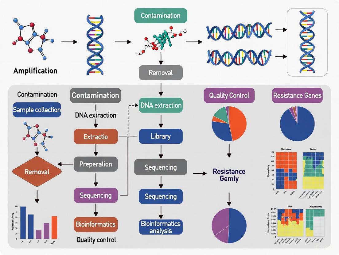
The following diagram outlines a robust workflow for metagenomic ARG analysis, integrating steps for contamination mitigation.
Diagram: Integrated ARG Analysis Workflow with Key Control Points.
Key Environmental Factors and Their Impact on ARG Abundance
Table: Key Environmental Drivers of ARG Abundance and Their Proposed Mechanisms [1] [3] [7].
| Environmental Factor | Observed Correlation with ARGs | Proposed Mechanism |
|---|---|---|
| Nutrients (N & P) | Strong positive correlation; Total Nitrogen (TN) identified as a major contributor [1]. | Nutrient pollution can enhance microbial growth and density, facilitating horizontal gene transfer and co-selection of ARGs. |
| Heavy Metals | Positive correlation with metals like Sb, Cu, Zn in mining areas [3]. | Co-selection where metal resistance genes (e.g., on same plasmid as ARGs) are selected for under metal stress. |
| pH | Significant correlation with tetracycline resistance genes (e.g., tetM) in soils [1]. | pH influences microbial community structure and the bioavailability of antibiotics and metals, indirectly shaping the resistome. |
| Antibiotic Residues | Direct selective pressure; water column antibiotics majorly affect sediment ARGs [1]. | Direct selection for bacteria possessing ARGs that confer resistance to the specific antibiotic present. |
| Mobile Genetic Elements | Strong co-occurrence network between ARGs and MGEs [6] [7]. | MGEs (plasmids, integrons, transposons) are the primary vectors for the horizontal transfer of ARGs between bacteria. |
Research Reagent Solutions
Table: Essential Tools and Databases for Contamination-Aware Metagenomic ARG Analysis.
| Reagent / Resource | Type | Primary Function in ARG Analysis |
|---|---|---|
| SARG+ [2] | ARG Database | A manually curated database that includes multiple variants per ARG from different species, improving detection accuracy and reducing false negatives. |
| GTDB [2] | Taxonomic Database | A comprehensive and quality-controlled taxonomic database used for accurate classification of microbial hosts, especially in long-read analysis. |
| ARGem Pipeline [4] | Bioinformatics Pipeline | A user-friendly, full-service pipeline that integrates ARG annotation with metadata capture and supports various visualizations, promoting reproducible and comparable results. |
| Argo Profiler [2] | Bioinformatics Tool | A tool specifically designed for long-read metagenomic data that uses read-overlapping and cluster-based classification to achieve highly accurate species-level host attribution of ARGs. |
| CARD / NDARO [2] | ARG Database | Widely used reference databases for antibiotic resistance. Often used in combination with other tools to ensure comprehensive ARG profiling. |
| Negative Control Samples | Wet-lab Control | Field and extraction blanks are processed alongside samples to identify and bioinformatically subtract laboratory and reagent-derived contaminants. |
| Unique Dual Indexes | Sequencing Reagent | Barcodes used during library preparation to minimize index hopping and cross-contamination between samples in a sequencing run. |
Troubleshooting Guides and FAQs
Environmental Cross-Talk
What is "environmental cross-talk" and how does it affect my metagenomic data?
Environmental cross-talk, or well-to-well contamination, occurs when genetic material from one sample inadvertently transfers to another during laboratory processing. This is not just background reagent contamination but represents a previously undocumented form of contamination where sequences from high-biomass samples appear in neighboring low-biomass samples [8]. This contamination primarily occurs during DNA extraction rather than PCR and is highest with plate-based methods compared to single-tube extraction [8]. The effect is most pronounced in low-biomass samples, where it can disproportionately impact alpha and beta diversity metrics and lead to incorrect ecological interpretations [8].
How significant is the distance effect for cross-contamination between samples?
Cross-contamination follows a distinct distance-decay relationship, with the highest rates occurring in immediately proximate wells [8]. Research has demonstrated that well-to-well contamination occurs primarily in neighboring samples, with rare events detected up to 10 wells apart [8]. The effect is more strongly distance-dependent for plate-based extractions than for manual single-tube methods [8].
Table 1: Well-to-Well Contamination Statistics by Extraction Method
| Extraction Method | Primary Contamination Source | Contamination Pattern | Distance Decay Relationship |
|---|---|---|---|
| Plate-Based Methods | DNA extraction process [8] | Highest in immediate neighbors, up to 10 wells away [8] | Stronger distance-decay effect [8] |
| Single-Tube Methods | DNA extraction process [8] | More dispersed pattern [8] | Weaker distance-decay effect [8] |
Recommended Protocol: Minimizing Environmental Cross-Talk
- Sample Randomization: Randomize samples across plates instead of grouping them by sample type or biomass. This prevents systematic bias from high-biomass samples contaminating entire groups of low-biomass samples [8].
- Biomass Grouping: When possible, process samples of similar biomasses together on the same plate [8].
- Physical Separation: Incorporate blank wells between samples, especially between high-biomass and low-biomass samples, to act as buffers [8].
- Method Selection: For critical low-biomass work, employ manual single-tube extractions or hybrid plate-based cleanups to reduce cross-talk compared to automated plate-based systems [8].
Laboratory Procedures
At which stage of my workflow is contamination most likely to occur?
Contamination can be introduced at virtually every stage, from sample collection to data analysis [9]. Major sources during laboratory procedures include:
- Sample Collection: Contamination from human operators, sampling equipment, and adjacent environments [9].
- DNA Extraction: This is a critical point for well-to-well contamination in plate-based formats [8]. It also introduces contaminants from reagents and kits [9].
- Library Preparation: While less frequent than during extraction, cross-contamination can also occur in this stage [8].
Human-derived contamination primarily comes from the laboratory personnel themselves. Sources include aerosol droplets from breathing or talking, as well as cells shed from clothing, skin, and hair [9]. Poor aseptic technique, such as talking over open samples, resting pipettes on benches, or wearing the same personal protective equipment (PPE) between different samples, are classic examples of lapses that lead to contamination [10].
Recommended Protocol: Contamination-Control During Lab Work
- Personal Protective Equipment (PPE): Wear appropriate PPE—including gloves, lab coats, goggles, and—for very low-biomass work—face masks and hair covers to create a barrier between the operator and the sample [9].
- Aseptic Technique: Use sterile, single-use consumables wherever possible. Decontaminate work surfaces and equipment with solutions like ethanol (to kill microbes) followed by a nucleic acid degrading solution like bleach (to remove DNA residues) before and after use [9].
- Workflow Design: Implement a one-way workflow where samples and reagents move from "clean" areas (e.g., sample preparation and PCR setup) to "dirty" areas (e.g., post-amplification analysis) without backtracking [10].
- Equipment Maintenance: Regularly clean and calibrate equipment. Use HEPA-filtered laminar flow hoods or biological safety cabinets for sensitive steps [10].
Reagent Microbiomes
What is meant by the "reagent microbiome"?
The "reagent microbiome" refers to the background microbial DNA present in the reagents and consumables (e.g., DNA extraction kits, plasticware, water, and PCR master mix) used in laboratory workflows [8]. This DNA is co-extracted and co-amplified with the target DNA from your sample, contributing a contaminant "noise" that can be particularly problematic in low-biomass studies where the contaminant signal can overwhelm the true biological signal [9].
How can I identify contaminants from my reagent microbiome?
The most effective method is the consistent use of negative controls (or "blanks") throughout your workflow. These controls should undergo the exact same processing as your samples—from DNA extraction to sequencing—but contain no template biological material [9]. The sequences identified in these negative controls represent your specific reagent and laboratory contaminant profile.
Table 2: Essential Controls for Contamination Identification
| Control Type | Composition | Purpose | What It Identifies |
|---|---|---|---|
| Negative Control (Blank) | No-template sample (e.g., sterile water) taken through entire workflow [9] | Defines the background contaminant profile | Reagent contaminants, laboratory environment contaminants [9] |
| Positive Control | Known community (Mock community) or single organism [9] | Verifies assay sensitivity and specificity | PCR inhibition, protocol failures, bioinformatic errors [9] |
| Sampling Control | Swab of air, PPE, or sampling equipment [9] | Identifies contamination introduced during sample collection | Contamination from the sampling environment or personnel [9] |
Recommended Protocol: Managing Reagent Microbiome Effects
- Batch Testing: If possible, test different lots of extraction kits to select those with the lowest background contamination for your specific application [11].
- Use Certified Kits: Choose DNA extraction kits that are manufactured according to high standards and are recommended for low-biomass work [11].
- Critical Interpretation: Be cautious with simplistic bioinformatic approaches that remove all taxa found in negative controls. This can be misleading, as sequences in blanks may be due to cross-talk from other samples rather than just reagent contaminants [8].
- Ultra-Clean Reagents: For extremely sensitive applications, reagents can be treated with UV sterilization or DNase to degrade contaminating DNA, or purchased as certified DNA-free [9].
The Scientist's Toolkit: Essential Research Reagents & Materials
Table 3: Key Reagent and Material Solutions for Mitigating Contamination
| Item | Function | Considerations for Low-Biomass Studies |
|---|---|---|
| PureLink Microbiome DNA Purification Kit (example) | DNA extraction from various sample types using a triple lysis approach (beads, heat, chemicals) for efficient microbial cell wall disruption [11] | Includes a clean-up buffer to remove inhibitors; manufacturers should follow high production standards to minimize kit-borne contaminants [11]. |
| Pre-sterilized Consumables | Single-use, DNA-free pipette tips, tubes, and plates act as physical barriers to contaminants [10]. | Eliminates variability and effort of in-house cleaning. Using plates with individual tube strips may reduce well-to-well contamination compared to fixed-well plates [8]. |
| DNA Degrading Solutions (e.g., Bleach, DNA Away) | Chemical sterilants used to decontaminate surfaces and equipment by degrading trace DNA [9] [10]. | Critical for removing cell-free DNA that remains after ethanol treatment or autoclaving. Use on lab benches, instruments, and reusable equipment [9]. |
| HEPA-Filtered Laminar Flow Hood/BSC | Provides a sterile, particle-free air environment for handling samples and setting up sensitive reactions like PCR [10]. | Protects against airborne contaminants and aerosols. Essential for processing low-biomass samples and setting up library preparations [10]. |
| Qubit Fluorometer | Provides highly accurate and specific quantification of DNA concentration using fluorescent dyes [11]. | More accurate for microbiome samples than spectrophotometers (e.g., NanoDrop), which can overestimate concentration due to contaminants [11]. |
The analysis of antibiotic resistance genes (ARGs) in hyper-eutrophic lakes reveals distinct profiles shaped by anthropogenic contamination. Below are consolidated findings from relevant case studies.
Table 1: ARG Distribution and Abundance in Hyper-Eutrophic Lakes
| Lake / Study | Predominant ARG Types (% of Total) | Primary Bacterial Hosts (Carrying ARGs) | Key Anthropogenic Influences |
|---|---|---|---|
| Lake Cajititlán, Mexico [12] | Multidrug (63.33%), Macrolides (11.55%), Aminoglycosides (8.22%), Glycopeptides (6.22%), Tetracyclines (4%) | Pseudomonas (144 genes), Stenotrophomonas (88 genes), Mycobacterium (54 genes) | Urban wastewater, agricultural and livestock runoff [12] |
| Chaohu Lake, China [13] | Multidrug, Bacitracin, Polymyxin, Macrolide-Lincosamide-Streptogramin (MLS), Aminoglycoside | Proteobacteria, Actinobacteria, Cyanobacteria, Firmicutes, Bacteroidetes | Wastewater treatment plants, hospitals, agricultural activity, pesticides, PPCPs [13] [14] |
| ~350 Canadian Lakes [15] | Vast diversity of naturally occurring ARGs, with significant impact from human activity. | Not Specified | Watershed agriculture/pasture, manure fertilizer, wastewater effluent, population density, number of hospitals [15] |
Table 2: Key Physicochemical Factors Influencing ARG Profiles
| Factor | Correlation/Influence on ARGs | Supporting Study |
|---|---|---|
| Total Phosphorus (TP) / PO₄-P | Strong positive correlation (0.4971 for TP, 0.5927 for PO₄-P). Key indicator of eutrophication's link to ARG abundance [13]. | Chaohu Lake [13] |
| Nutrients (Nitrogen) | Lesser, but measurable impact (Total Nitrogen: 0.0515) compared to phosphorus [13]. | Chaohu Lake [13] |
| Pesticides & PPCPs | Act as co-selectors for antibiotic resistance, facilitating ARG transfer even at sub-inhibitory concentrations [14]. | Chaohu Lake [14] |
| Trophic Status | Increasing eutrophication correlates with higher ARG abundance and diversity [15]. | Canadian Lakes Survey [15] |
Technical Support: Troubleshooting Contamination in Low-Biomass Metagenomics
Frequently Asked Questions (FAQs)
Q1: Our negative controls show high microbial biomass. What are the most likely sources of this contamination? A1: Contamination in low-biomass samples like oligotrophic lake water typically originates from:
- Reagents and Kits (Kitome): DNA extraction kits, polymerases, and water are common sources of contaminating microbial DNA. Different lots from the same manufacturer can have varying contaminant profiles [9] [16].
- Laboratory Environment: Human-associated microbiota from skin and hair, as well as aerosols from lab surfaces and air, can introduce contaminant DNA [9].
- Cross-Contamination: During sample processing, DNA can leak between adjacent samples in plates, or equipment used for multiple samples can be a vector if not properly decontaminated [9].
Q2: How can we distinguish true environmental ARG signals from contamination? A2: Distinguishing signal from noise requires a multi-pronged approach:
- Robust Negative Controls: Include "field blanks" (e.g., sterile water exposed to the sampling air) and "extraction blanks" (no-sample controls carried through DNA extraction) in every batch. The contaminant profiles from these controls should be bioinformatically subtracted from your actual samples [9].
- Statistical & Bioinformatic Decontamination: Use tools like
decontam(R package) which can identify contaminant sequences based on their higher prevalence in negative controls and/or their inverse correlation with DNA concentration [9]. - Consistency Across Replicates: True signals should be reproducible across your true sample replicates and correlate with expected environmental gradients [16].
Q3: Our metagenomic data is dominated by host (e.g., human) DNA from sampling. How can we mitigate this? A3: Host DNA depletion is critical for increasing the sequencing depth of your target microbiome.
- During Wet Lab: Use PPE (gloves, masks, coveralls) rigorously to minimize operator contamination. Decontaminate all sampling equipment with ethanol followed by a DNA-degrading solution (e.g., bleach, UV-C light) to remove residual DNA [9] [17].
- During Analysis: Bioinformatic host removal is a standard and essential step. After quality control, map your sequencing reads to a host reference genome (e.g., human GRCh38) and remove all matching reads before downstream assembly and analysis [17] [18].
Essential Methodologies & Protocols
Protocol 1: Contamination-Aware Sample Collection for Lake Water [9]
- Decontaminate Equipment: Treat samplers, bottles, and filters with 80% ethanol (to kill cells) followed by a nucleic acid degrading solution like 10% sodium hypochlorite (to remove DNA). Use DNA-free, single-use equipment where possible.
- Use Personal Protective Equipment (PPE): Wear gloves, masks, and clean suits to prevent contamination from the researcher.
- Collect Controls: Simultaneously collect multiple negative controls:
- Field Blank: Pass sterile, DNA-free water through a filter at the sampling site.
- Equipment Blank: Swab the sampling equipment.
- Air Blank: Leave an open, sterile Petri dish with a filter at the sampling site.
- Preserve Immediately: Flash-freeze filters in liquid nitrogen or at -80°C to halt biological activity.
Protocol 2: Bioinformatic Host DNA Removal and Quality Control [18] This protocol assumes you have paired-end metagenomic sequencing data.
- Quality Control (QC) & Trimming:
- Use
fastporTrimmomaticto remove adapter sequences and low-quality bases. - Run
FASTQCbefore and after trimming to visualize the quality of your data. - Code Example (fastp):
- Use
- Host Read Removal:
- Download a host reference genome (e.g., human GCF_000001405.26).
- Align your quality-filtered reads to the host genome using
Bowtie2and retain only the UNMAPPED reads. - Code Example (Bowtie2):
- The resulting
sample_nonhost.1.fastq.gzandsample_nonhost.2.fastq.gzfiles are your cleaned metagenomic data, ready for assembly and ARG analysis.
Protocol 3: Metagenome-Assembled Genome (MAG) Construction and ARG Profiling [18]
- Metagenomic Assembly: Assemble the cleaned, non-host reads into contigs using a metagenomic assembler like
MEGAHITormetaSPAdes.- Code Example (MEGAHIT):
- Binning: Group contigs into draft genomes (MAGs) using binning software like
metaWRAPbinning module. - Bin Refinement and Quality Check: Use
metaWRAPrefine module orDAS_Toolto obtain high-quality MAGs. Check completeness and contamination withCheckMorCheckM2. - Taxonomic Classification: Classify MAGs using
GTDB-Tk. - Functional Profiling & ARG Identification: Annotate genes on contigs or MAGs using
Prokka. Scan for ARGs using thestaramrtool or by aligning to databases like CARD (Comprehensive Antibiotic Resistance Database).
The Scientist's Toolkit: Key Research Reagent Solutions
Table 3: Essential Materials and Bioinformatics Tools for Metagenomic ARG Analysis
| Item / Solution | Function / Purpose | Example Tools / Brands |
|---|---|---|
| DNA-Free Collection Kits | Single-use, sterile filters and vessels to minimize contamination at source. | DNA-free water sampling kits, sterile disposable filter units [9]. |
| Nucleic Acid Degrading Solution | Destroys contaminating free DNA on equipment and surfaces post-ethanol decontamination. | Dilute sodium hypochlorite (bleach), commercial DNA removal solutions [9]. |
| High-Sensitivity DNA Extraction Kits | To extract maximum DNA from low-biomass samples while minimizing reagent-derived contaminant DNA. | QIAGEN DNeasy PowerWater Kit (used in Canadian Lake survey) [15]. |
| Sequence Data QC & Trimming | Assess read quality and remove adapters/ low-quality bases. | Fastp, FASTQC, Trimmomatic [17] [18]. |
| Host DNA Removal (Bioinformatic) | In-silico subtraction of host-associated reads to enrich for microbial data. | Bowtie2, BWA (for alignment to host genome) [17] [18]. |
| Metagenomic Assembler | Reconstructs longer DNA sequences (contigs) from short sequencing reads. | MEGAHIT, metaSPAdes [18]. |
| Metagenomic Binning Tool | Groups assembled contigs into draft genomes (MAGs) based on sequence composition and abundance. | metaWRAP, MaxBin2 [18]. |
| ARG Profiling Tool | Identifies and annotates antibiotic resistance genes from metagenomic data. | staramr (based on CARD, ResFinder, PointFinder) [18]. |
The Role of Mobile Genetic Elements (MGEs) in Misleading ARG Attribution
Troubleshooting Guide: Frequent Issues in Metagenomic ARG Analysis
Why am I detecting ARGs in samples where known resistant pathogens are absent?
This is a classic sign of MGE-mediated contamination or misattribution.
- Root Cause: ARGs are often embedded within Mobile Genetic Elements (MGEs) like plasmids, transposons, and integrons [19]. These elements can exist in a cell independently of the chromosome and are highly mobile between different bacterial species via Horizontal Gene Transfer (HGT) [19] [20].
- Solution:
- Re-analysis with Host Attribution: Use analytical tools that can link the detected ARG to its specific genetic context (e.g., is it on a plasmid or chromosome?) and to a taxonomic host [21].
- Profile MGE Co-occurrence: Actively map the abundance of MGEs in your sample. A strong correlation between the abundance of a specific ARG and specific MGEs is a strong indicator of potential HGT and misattribution [22] [20].
- Employ Long-Read Sequencing: Technologies like Oxford Nanopore or PacBio generate long sequences that can span an ARG and its adjacent genetic elements, providing clearer evidence of the host species and the mobile nature of the gene [21].
Why do I get inconsistent ARG host identification between replicate experiments?
Inconsistencies often stem from the dynamic nature of MGEs and limitations in short-read sequencing.
- Root Cause: MGEs can be gained or lost by bacterial cells without affecting their core genomic identity. Short-read metagenomic sequencing often produces fragmented data, making it difficult to correctly assemble the full context of an ARG, leading to variable host assignments across runs [21].
- Solution:
- Utilize Advanced Profiling Tools: Implement methods like Argo, which uses long-read overlapping to cluster ARG-containing reads before taxonomic assignment. This collective labeling of read clusters significantly improves the accuracy and consistency of host identification compared to per-read classification [21].
- Strict Contamination Control: Follow a strict experimental guideline to rule out technical contamination from reagents or lab equipment, which can introduce exogenous genetic material [23].
How can I distinguish a genuine chromosomal ARG from a plasmid-borne one?
Determining the genetic location is crucial for assessing the transfer risk of an ARG.
- Root Cause: Plasmids are a major type of MGE and primary vectors for the rapid dissemination of ARGs across bacterial populations [19] [20].
- Solution:
- Database Mapping: Map your metagenomic reads not only to ARG databases but also to dedicated plasmid databases (e.g., a decontaminated subset of RefSeq plasmid) [21].
- Contextual Analysis: Look for genetic signatures of plasmids or other MGEs in the sequences flanking the detected ARG. The presence of mobility genes (e.g., transposases, integrases) is a key indicator [22] [19].
The following table summarizes key types of Mobile Genetic Elements and their documented impact on ARG dissemination as observed in recent environmental metagenomic studies.
Table 1: Mobile Genetic Elements (MGEs) and Their Documented Role in ARG Dissemination
| MGE Type | Key Characteristics | Primary Mechanism in ARG Spread | Documented Findings |
|---|---|---|---|
| Plasmids [19] [20] | Extrachromosomal DNA elements; can be conjugative. | Conjugation between bacterial cells. | Carry a wide variety of bla (β-lactamase) and erm (macrolide resistance) genes; lead to co-selection of multiple resistance traits [19]. |
| Transposons (Tn) & Composite Transposons (ComTn) [19] [20] | DNA sequences that can move within the genome. | Transposition within a cell's DNA; can be carried by plasmids. | Frequently associated with ARGs; ComTn can mobilize nearby genes, facilitating their spread to other MGEs [20]. |
| Insertion Sequences (IS) [19] [20] | Simplest transposable elements (<3 kb); encode transposase. | Transposition; can inactivate genes or provide promoters. | High copy numbers in genomes; can mediate mobilization of adjacent genes, contributing to the formation of ComTn [19] [20]. |
| Integrative & Conjugative Elements (ICEs) [20] | Integrate into the chromosome but can excise and conjugate. | Conjugation, similar to plasmids. | Can carry intracellular transposing MGEs and ARGs, acting as a bridge for gene transfer between integrated and mobile states [20]. |
| Integrons [19] | Site-specific recombination systems that capture gene cassettes. | Capture and promote expression of antibiotic resistance genes. | Often located within transposons and plasmids; enable bacteria to rapidly acquire and stack multiple resistance genes [19]. |
Detailed Experimental Protocol: Tracking MGE-Mediated ARG Transfer
This protocol outlines a metagenomic approach to identify ARGs and their associated MGEs in complex environmental samples, helping to clarify their origins and dissemination pathways.
Sample Collection and DNA Extraction
- Sample Type: The protocol can be applied to water samples (e.g., from lakes or sewage) [22] [20] or other environmental matrices.
- Microbial Enrichment: Filter water samples through membranes to concentrate microbial biomass [22].
- DNA Extraction: Use a standard phenol-chloroform method or commercial kit to extract total microbial DNA [22]. The extraction should be optimized for high molecular weight DNA if long-read sequencing is planned.
Metagenomic Sequencing and Data Processing
- Sequencing Platform: Use either:
- Quality Control: Process raw reads with tools like Fastp to remove low-quality sequences and adapters [22].
- Assembly: For short-read data, assemble clean reads into contigs using MEGAHIT or similar assemblers [22].
Gene Prediction and Annotation
- Open Reading Frame (ORF) Prediction: Use Prodigal to predict protein-coding genes on the assembled contigs or directly on long reads [22].
- ARG Identification: Annotate ARGs using the DeepARG-LS model to achieve high accuracy and low false-negative rates [22]. The reference database SARG+, which consolidates and expands sequences from CARD, NDARO, and SARG, is recommended for comprehensive profiling [21].
- MGE Annotation: Annotate MGEs by aligning ORFs to a specialized database like the mobileOG-DB [22].
- MRG Annotation: Align ORFs to the BacMet database to identify metal resistance genes, which can be co-selected with ARGs [22].
Identification of ARG Hosts and Dissemination Risk
- Taxonomic Assignment: Assign taxonomy to ARG-containing sequences by aligning them to a curated database like GTDB using BLAST or minimap2 [22] [21].
- Correlation and Network Analysis: Use correlation algorithms (e.g., SparCC) to identify significant positive correlations between the abundance profiles of specific ARGs, MGEs, and bacterial taxa [20]. This helps identify potential hosts and vectors.
- Risk Assessment: Tools like MetaCompare can be used to assess the potential dissemination risk of ARGs based on the co-occurrence of acquired ARGs, human bacterial pathogens (HBPs), and MGEs [22].
Visualizing the Workflow for Contamination-Aware ARG Analysis
The following diagram illustrates the core logical workflow for conducting a metagenomic analysis that accounts for MGEs to prevent misattribution of ARGs.
The Scientist's Toolkit: Essential Research Reagents & Databases
Table 2: Key Bioinformatics Tools and Databases for ARG and MGE Analysis
| Resource Name | Type | Primary Function | Key Application in Mitigating Misattribution |
|---|---|---|---|
| DeepARG-LS [22] | Computational Tool / Model | Accurate annotation of antibiotic resistance genes from metagenomic data. | Reduces false positives/negatives in initial ARG detection, providing a more reliable foundation for analysis. |
| SARG+ [21] | Manually Curated Database | A comprehensive compendium of ARG protein sequences, expanded from CARD, NDARO, and SARG. | Includes ARG variants from multiple species, improving detection sensitivity and reducing misattribution due to sequence divergence. |
| mobileOG-DB [22] | Database | An integrated database of protein sequences for annotating Mobile Genetic Elements. | Allows for the systematic identification of MGEs in metagenomes, enabling the study of their correlation with ARGs. |
| BacMet [22] | Database | A database of experimentally verified biocide and metal resistance genes. | Identifying metal resistance genes helps reveal co-selection pressures that may maintain ARGs in the absence of direct antibiotic selection. |
| Argo [21] | Computational Profiler | Species-resolved ARG profiling from long-read metagenomes using read-overlapping and clustering. | Dramatically improves the accuracy of host identification by collectively labeling read clusters, directly addressing the misattribution problem. |
| GTDB (Genome Taxonomy Database) [21] | Database | A high-quality, standardized bacterial and archaeal taxonomy. | Provides a reliable reference for taxonomic classification, reducing errors in host assignment from sequence data. |
Impact of Contamination on Resistome Risk Assessment and Data Interpretation
Frequently Asked Questions (FAQs)
FAQ 1: What are the most common sources of contamination in metagenomic studies for antibiotic resistome risk assessment? Contamination can originate from multiple sources throughout the experimental workflow. Key sources include:
- Reagents and Kits: DNA extraction kits and polymerase enzymes often contain microbial DNA, creating a unique "kitome" background that varies between brands and even between lots of the same product [24] [16].
- Laboratory Environment: Contaminants can be introduced from laboratory surfaces, air, and equipment [9] [16].
- Sample Handling: Human skin of operators, improper sterile technique, and cross-contamination between samples during processing are significant sources [9] [16].
- Sequencing Process: Index hopping in multiplexed runs and well-to-well leakage during library preparation can cause cross-contamination [24].
FAQ 2: How does contamination specifically impact the assessment of antibiotic resistance gene (ARG) risk? Contamination skews risk assessment by distorting key metrics:
- False Positives: It can lead to the false detection of high-risk ARGs and human bacterial pathogens (HBPs), resulting in an overestimation of the resistome risk [24] [25].
- Distorted Abundance and Diversity: Contaminant sequences artificially inflate the perceived abundance and diversity of ARGs, complicating ecological interpretations [26] [27].
- Compromised Connectivity Analysis: Accurate tracking of ARG transfer between environmental and clinical settings depends on distinguishing true signals from background noise. Contamination obscures these pathways [27].
FAQ 3: What are the best practices for preventing and controlling contamination during sample collection and processing? A contamination-informed sampling design is critical [9]. Key practices include:
- Decontamination: Thoroughly decontaminate equipment and surfaces with 80% ethanol followed by a nucleic acid-degrading solution (e.g., bleach) [9].
- Personal Protective Equipment (PPE): Use gloves, lab coats, masks, and hair covers to minimize contamination from operators [9].
- Use of Controls: Always include negative controls (e.g., extraction blanks with molecular-grade water) and sampling controls (e.g., swabs of the air or sampling surfaces) in every run [9] [24].
- Reagent Quality: Use high-quality, trusted reagents and consider aliquoting to minimize repeated exposure [28].
FAQ 4: My negative controls show microbial signals. How should I handle this in my data analysis? The presence of signals in negative controls confirms the need for bioinformatic decontamination. You should:
- Profile the Contaminants: Use the negative controls to create a profile of the background "kitome" and laboratory contaminants [24].
- Apply Statistical Tools: Utilize specialized bioinformatics tools like
Decontam(which identifies contaminants based on their higher frequency in low-concentration samples and negative controls),SourceTracker, ormicroDeconto statistically identify and remove contaminant sequences from your dataset [24]. - Report the Process: Transparently report the contamination profiles and the decontamination steps taken in your methodology [9].
FAQ 5: Are some sequencing approaches more robust against contamination for resistome risk assessment? Emerging methods are being developed to improve accuracy. Long-read sequencing (e.g., Nanopore, PacBio) offers advantages by allowing for the analysis of ARGs, mobile genetic elements (MGEs), and their hosts without assembly, reducing chimeric artifacts [25]. Specifically, the Long-read based Antibiotic Resistome Risk Assessment Pipeline (L-ARRAP) has been developed to quantify ARG risk from long-read data, helping to distinguish true genetic linkages from spurious ones [25].
Quantitative Data on Contamination Impacts
Table 1: Documented Impacts of Contaminants on Resistome Profiles
| Contaminant Source | Observed Impact on Resistome Analysis | Study Context |
|---|---|---|
| DNA Extraction Reagents | Distinct background microbiota profiles found across commercial brands; patterns varied significantly between different lots of the same brand [24]. | Clinical mNGS for pathogen detection [24]. |
| Landfill Leachate (as an environmental contaminant) | Elevated levels of ARGs (e.g., sul, tet) and heavy metals found; metal pollution suggested to co-select for antibiotic resistance [26]. |
Metagenomic analysis of landfill leachates [26]. |
| Global Soil Resistome | Analysis showed soil shares 50.9% of its high-risk Rank I ARGs with human-associated habitats like feces and wastewater, highlighting connectivity and potential cross-contamination [27]. | Global meta-analysis of soil metagenomes [27]. |
Table 2: Key Metrics for High-Risk ARG (Rank I) Assessment [27]
| Metric | Definition | Interpretation |
|---|---|---|
| Relative Abundance | Copies of Rank I ARGs per 1000 cells. | Measures the prevalence of high-risk genes within a microbial community. |
| Occurrence Frequency | Proportion of samples in a set where a specific ARG is detected. | Indicates how widespread a high-risk ARG is across different samples. |
| Connectivity | Genetic overlap of ARGs with clinical pathogens, assessed through sequence similarity and phylogenetic analysis. | Evaluates the potential transfer risk of ARGs from the environment to human pathogens. |
Essential Experimental Protocols
Protocol 1: Implementing Negative and Process Controls
Purpose: To identify and account for background contamination introduced from reagents and the laboratory environment [9] [24].
Detailed Methodology:
- Extraction Blank: For each batch of DNA extractions, include a sample where molecular biology-grade water is used as the input instead of a biological sample. Process this blank identically to all other samples [24].
- Sampling Controls: During field sampling, include controls such as:
- An empty, sterile collection vessel exposed to the air.
- A swab of the air at the sampling site.
- A swab of the gloves or PPE of the sampler [9].
- Processing: Subject all controls to the entire downstream workflow, including DNA extraction, library preparation, and sequencing, alongside the actual samples.
- Analysis: Use the sequencing data from these controls to create a contaminant profile for your specific study, which can then be used for bioinformatic decontamination [24].
Protocol 2: Bioinformatics Decontamination withDecontam
Purpose: To statistically identify and remove contaminant sequences from metagenomic data [24].
Detailed Methodology:
- Data Input: Prepare a feature table (e.g., ASV or OTU table) and a corresponding table of sequence metadata.
- Identify Contaminants: Use the
Decontampackage in R with the "prevalence" method. This method identifies contaminants as sequences that are significantly more prevalent in negative control samples than in true biological samples. - Threshold Setting: Apply a user-defined probability threshold (e.g., 0.5) to classify features as contaminants.
- Data Filtering: Remove the identified contaminant sequences from the feature table and all downstream analyses.
- Validation: Compare the community composition and ARG profiles before and after decontamination to ensure realistic outcomes.
Protocol 3: Assessing ARG Risk with the L-ARRAP Pipeline
Purpose: To quantify the antibiotic resistome risk in metagenomic samples, particularly those from long-read sequencing platforms [25].
Detailed Methodology:
- Quality Control: Process raw long-reads (Nanopore/PacBio) with a tool like
Chopper, using parameters such as-q 10 -l 500to filter out low-quality and short reads [25]. - ARG and MGE Identification: Align quality-controlled reads to the SARG database for ARGs and the MobileOG-db for mobile genetic elements (MGEs). Use
Minimap2for ARGs andLASTfor MGEs, with thresholds of >75% identity and >90% coverage [25]. - Pathogen Identification: Annotate the taxonomy of reads using
Centrifugeand identify reads belonging to Human Bacterial Pathogens (HBPs) by comparing them to a curated database from WHO and ESKAPE pathogens [25]. - Calculate Risk Index: The Long-read based Antibiotic Resistome Risk Index (L-ARRI) is calculated by integrating the abundance of ARGs, their mobility potential (link to MGEs), and their association with pathogenic hosts [25].
Workflow Diagrams
Diagram 2: L-ARRAP Risk Assessment Pipeline for Long Reads
The Scientist's Toolkit: Essential Reagents & Solutions
Table 3: Key Research Reagent Solutions for Contamination Control
| Item | Function/Purpose | Key Considerations |
|---|---|---|
| Molecular Grade Water | Used for preparing solutions and as input for extraction blanks. Must be DNA-/RNA-free and nuclease-free [24]. | Verify sterility and the absence of microbial bioburden. Pre-filtration (0.1 µm) is a key quality indicator [24]. |
| DNA Decontamination Solutions | Used to remove contaminating DNA from surfaces and equipment before use. | Sodium hypochlorite (bleach), UV-C light, hydrogen peroxide, or commercial DNA removal solutions are effective [9]. |
| High-Fidelity Polymerases | Enzymes for PCR and library amplification with low levels of contaminating DNA. | Recombinant polymerases generally have lower contamination, but levels should be checked. Avoid enzymes with known viral contaminants [16]. |
| Spike-in Controls | Synthetic microbial communities (e.g., ZymoBIOMICS Spike-in Control) added to samples. | Serves as an internal positive control for extraction and sequencing efficiency, helping to distinguish technical failures from true negatives [24]. |
| Mycoplasma Prevention & Detection Kits | To prevent and detect mycoplasma contamination in cell cultures used for experiments. | Regular testing (every 1-2 months) is recommended. Use removal reagents and prevention sprays for contaminated cultures [28]. |
Advanced Profiling and Source Tracking: Cutting-Edge Methodologies for Accurate ARG Detection
Species-Resolved ARG Profiling with Long-Read Sequencing Technologies
Antimicrobial resistance (AMR) poses a critical global health threat, directly responsible for an estimated 1.14 million deaths worldwide in 2021 alone, with projections rising to 1.91 million by 2050 without concerted global action [21]. Environmental surveillance of antibiotic resistance genes (ARGs) is crucial for understanding and mitigating the spread of antimicrobial resistance. While metagenomic sequencing has revolutionized AMR surveillance by enabling culture-free analysis of complex microbial communities, traditional short-read technologies have faced significant limitations in linking detected ARGs to their specific microbial hosts—information indispensable for tracking transmission and assessing risk [21] [29].
Long-read sequencing technologies from platforms such as Oxford Nanopore Technologies (ONT) and PacBio have emerged as powerful solutions for overcoming these challenges. These technologies generate reads tens of thousands of bases in length, enabling them to span not only full-length ARGs but also their surrounding genomic context [21]. This contextual information dramatically increases the likelihood of correct taxonomic classification and provides insights into whether ARGs are located on chromosomes or mobile genetic elements—a critical distinction for assessing transmission risk [30].
This technical support center provides comprehensive guidance for researchers implementing long-read sequencing for species-resolved ARG profiling, with particular emphasis on mitigating contamination and analytical artifacts in metagenomic analysis. The protocols and troubleshooting guides below address common experimental and bioinformatic challenges to ensure accurate, reliable results.
Frequently Asked Questions (FAQs)
Q1: What are the primary advantages of long-read over short-read sequencing for ARG surveillance?
Long-read technologies provide two fundamental advantages for ARG profiling: (1) Enhanced host tracking: Reads spanning entire ARGs plus flanking regions enable more reliable taxonomic assignment to species level [21]; (2) Contextual information: Long reads can determine whether ARGs are located on chromosomes or mobile genetic elements like plasmids, informing mobility risk assessment [30]. Short-read approaches often fail to resolve these aspects due to fragmentation in complex genomic regions surrounding ARGs [29].
Q2: How does the Argo method improve accuracy in host identification compared to traditional approaches?
Argo employs a novel read-overlapping approach that clusters ARG-containing reads before taxonomic assignment, unlike tools like Kraken2 or Centrifuge that assign taxonomy to individual reads. By leveraging graph clustering of read overlaps and assigning taxonomic labels collectively to read clusters, Argo substantially reduces misclassifications that commonly occur with per-read methods, especially for ARGs prone to horizontal gene transfer that may appear across multiple species [21].
Q3: My metagenomic assemblies consistently break around ARG regions. Is this a technical issue?
Assembly fragmentation around ARGs is a recognized technical challenge, not necessarily an error in your workflow. ARGs are often surrounded by repetitive regions and mobile genetic elements, and nearly identical ARG variants can occur in multiple genomic contexts across different species. These factors create highly complex, branched assembly graphs that assemblers resolve by breaking them into shorter contigs [29]. Consider complementing assembly-based approaches with read-based methods like Argo for more accurate ARG quantification and host assignment [21] [29].
Q4: Can long-read sequencing detect resistance mechanisms beyond acquired ARGs, such as chromosomal mutations?
Yes. Recent advances enable long-read technologies to identify resistance-associated point mutations through haplotype phasing. For example, fluoroquinolone resistance mechanisms include both plasmid-mediated genes (qnrA, qnrB, qnrS) and chromosomal mutations in gyrA and parC genes. Specialized bioinformatic approaches can now uncover these strain-level SNPs directly from metagenomic data [30].
Q5: How can I distinguish genuine ARG hosts from false positives due to contamination?
Multiple strategies can mitigate false host assignments: (1) Implement read clustering approaches like Argo that reduce misclassification [21]; (2) Leverage DNA methylation signatures to link plasmids to their bacterial hosts based on common methylation patterns [30]; (3) Use coverage-based filters and read-pair consistency checks to eliminate chimeric neighborhoods, as implemented in tools like ARGContextProfiler [31].
Troubleshooting Guides
Common Experimental Challenges
Table 1: Troubleshooting Experimental Challenges
| Problem | Potential Causes | Solutions | Contamination Mitigation |
|---|---|---|---|
| Low ARG detection sensitivity | Inadequate DNA quantity/quality, low sequencing depth, inefficient library preparation | Use high molecular weight DNA extraction methods, increase sequencing depth, optimize library prep for complex samples | Include extraction controls to detect reagent contamination |
| Inaccurate host assignment | Sequencing errors, horizontal gene transfer events, database limitations | Apply adaptive identity cutoffs based on read quality, use clustering approaches like Argo, employ comprehensive databases like SARG+ [21] | Validate host assignments with complementary methods (e.g., methylation linking) [30] |
| Failure to detect plasmid-borne ARGs | Reference databases lacking plasmid sequences, incomplete assembly | Augment databases with plasmid sequences (e.g., RefSeq plasmid), implement methylation-based plasmid-host linking [30] | Use decontaminated plasmid databases to minimize false positives |
| Inconsistent results between replicates | Variable DNA extraction efficiency, sampling heterogeneity, sequencing batch effects | Standardize extraction protocols, increase biological replicates, randomize sequencing across batches | Monitor technical variation through process controls |
Bioinformatics and Analysis Challenges
Table 2: Troubleshooting Bioinformatics Challenges
| Problem | Diagnostic Steps | Solutions | Preventive Measures |
|---|---|---|---|
| Assembly fragmentation around ARGs | Check for repetitive regions flanking ARGs, assess coverage uniformity | Use specialized assemblers like Trinity or metaSPAdes, combine with read-based approaches [29] | Implement local assembly approaches or graph-based context extraction [31] |
| High false positive ARG calls | Verify alignment identity thresholds, check for regulator/housekeeping genes | Apply stringent identity cutoffs, use curated databases that exclude regulators and housekeeping genes [21] | Employ frameshift-aware alignment (DIAMOND) and filter non-bona fide ARGs [21] |
| Inability to resolve strain-level variation | Assess read length and coverage, check haplotype phasing capability | Implement strain haplotyping tools, leverage ultra-long phasing blocks [30] | Utilize technologies that maintain haplotype information (linked reads, phased sequencing) [32] |
| Chimeric genomic contexts | Examine assembly graph complexity, check for repetitive elements | Use ARGContextProfiler to validate contexts through read mapping and coverage consistency [31] | Apply graph-based approaches with multiple filters to eliminate chimeric paths |
Key Experimental Protocols
Argo Workflow for Species-Resolved ARG Profiling
The Argo methodology represents a significant advancement for accurate host tracking in long-read metagenomics [21]. The following protocol details its implementation:
Step 1: ARG Identification
- Begin with quality-controlled long reads from ONT or PacBio platforms
- Identify ARG-containing reads using DIAMOND's frameshift-aware DNA-to-protein alignment against the SARG+ database
- Set adaptive identity cutoff based on per-base sequence divergence derived from read overlaps
- Record ARGs with their precise coordinates on reads for downstream analysis
Step 2: Taxonomic Classification
- Map ARG-containing reads to the GTDB reference taxonomy database using minimap2's base-level alignment
- Generate candidate species labels for each read
- Aggregate labels into candidate species sets where each set contains at least one read
Step 3: Read Clustering
- Overlap ARG-containing reads to construct a sparse overlap graph representing pairwise identities
- Segment the graph into read clusters using the Markov Cluster (MCL) algorithm
- Refine taxonomic assignments on a per-cluster basis using greedy set covering
Step 4: Plasmid Detection
- Mark reads as "plasmid-borne" if they additionally map to a decontaminated subset of RefSeq plasmid database
- Exclude phage-associated ARGs as they rarely represent bona fide resistance genes
Argo Analysis Workflow
Methylation-Based Plasmid-Host Linking
This protocol leverages DNA modification detection in native long reads to associate plasmids with their bacterial hosts, addressing a key challenge in tracking ARG transmission [30]:
Step 1: Native DNA Sequencing
- Perform ONT sequencing without PCR amplification to preserve natural DNA modifications
- Use appropriate flow cells (R10 recommended) and chemistry (V14 or newer) for optimal modification detection
Step 2: Methylation Motif Detection
- Basecall raw signals with modified base detection enabled (e.g., Dorado with 5mC/6mA models)
- Identify methylation motifs using MicrobeMod or NanoMotif
- Generate per-sample methylation profiles for both chromosomal and plasmid reads
Step 3: Host-Linking Analysis
- Cluster plasmids and bacterial hosts based on shared methylation motifs
- Validate links using coverage correlation and sequence composition
- Resolve ambiguous assignments through manual inspection of motif conservation
Strain-Level Haplotyping for Point Mutation Detection
This protocol enables identification of resistance-conferring point mutations directly from metagenomic data [30]:
Step 1: Variant Calling
- Map long reads to reference genomes or MAGs using minimap2 or similar aligner
- Call variants with tools sensitive to metagenomic data characteristics
- Filter variants based on quality metrics and coverage thresholds
Step 2: Haplotype Phasing
- Phase variants into haplotypes using long-read connectivity
- Apply population genetics models to distinguish strains
- Validate phasing accuracy through comparison with isolate sequencing when available
Step 3: Mutation Annotation
- Annotate phased variants with functional prediction
- Cross-reference with known resistance mutations (e.g., gyrA for fluoroquinolone resistance)
- Correlate mutation patterns with ARG profiles for comprehensive resistome assessment
Research Reagent Solutions
Table 3: Essential Research Reagents and Databases
| Category | Resource | Function | Key Features | Contamination Control |
|---|---|---|---|---|
| ARG Databases | SARG+ [21] | Comprehensive ARG reference | Manually curated compendium from CARD, NDARO, SARG; excludes regulators/housekeeping genes | Deduplicated sequences; focused on bona fide ARGs |
| CARD [33] | ARG identification and annotation | Antibiotic Resistance Ontology; rigorous curation standards | Experimentally validated sequences only | |
| Taxonomy Databases | GTDB [21] | Taxonomic classification | Higher quality control than NCBI; better resolved taxonomy | Deprecated assemblies removed |
| NCBI RefSeq [21] | Reference sequences | Comprehensive collection including plasmids | Decontaminated subsets available | |
| Analysis Tools | Argo [21] [34] | Species-resolved ARG profiling | Read clustering approach; reduces misclassification | Adaptive identity cutoffs based on read quality |
| ARGContextProfiler [31] | Genomic context extraction | Assembly graph exploration; minimizes chimeric errors | Coverage-based filtering of false contexts | |
| NanoMotif [30] | Methylation motif detection | Plasmid-host linking via shared methylation patterns | Single-library approach reduces contamination risk | |
| Sequencing Technologies | ONT R10/V14 [30] | Long-read sequencing | Native DNA modification detection; improved accuracy | Preserves natural modification signatures |
| PacBio HiFi [32] | High-fidelity long reads | Circular consensus sequencing; high accuracy | Reduced systematic errors |
Advanced Technical Considerations
Mitigating Assembly Artifacts in ARG Regions
Metagenomic assemblies frequently break around ARGs due to their association with repetitive elements and multiple genomic contexts [29]. To address this:
Hybrid Assembly Approaches
- Combine long reads for scaffolding with short reads for base-level accuracy
- Use metaSPAdes or Trinity for improved recovery of ARG contexts compared to other assemblers
- Implement iterative assembly strategies focusing on ARG-containing regions
Graph-Based Context Extraction As implemented in ARGContextProfiler [31]:
- Extract ARG neighborhoods directly from assembly graphs before linearization
- Apply multiple filters (read-pair consistency, coverage variation) to eliminate chimeric paths
- Validate reconstructed contexts through independent read mapping
Quantitative Framework for ARG Source Tracking
Machine learning classification combined with comprehensive ARG profiling enables probabilistic source attribution [35]:
Implementation Steps
- Build reference ARG profiles from potential source environments (human/animal gut, wastewater, soil)
- Apply Bayesian classification tools (SourceTracker) to estimate source contributions in sink samples
- Identify specialist indicator ARGs specific to particular sources
- Validate predictions through artificial configurations with known source proportions
ARG Source Tracking Framework
Leveraging Tools like Argo for Enhanced Host Attribution and Read Clustering
Frequently Asked Questions (FAQs)
Q1: What is Argo and how does it improve upon existing methods for tracking Antibiotic Resistance Gene (ARG) hosts? Argo is a novel bioinformatics tool that uses long-read metagenomic sequencing to identify and quantify antibiotic resistance genes (ARGs) and accurately link them to their specific microbial hosts at the species level. Unlike short-read methods that often misattribute ARGs due to fragmented assemblies, Argo leverages long-read overlapping and graph-based clustering to collectively assign taxonomic labels to groups of reads, significantly enhancing the accuracy of host identification and providing superior resolution for tracking ARG transmission [21].
Q2: My analysis is plagued by high levels of contamination from off-target DNA. How can Argo help mitigate this? Argo's workflow includes a stringent, frameshift-aware alignment step to a manually curated ARG database called SARG+. This database excludes regulators, housekeeping genes, and ARGs from point mutations that are not direct indicators of antibiotic resistance. By using this focused database and applying adaptive identity cutoffs, Argo reduces false positives from non-target genetic material, ensuring that the reported ARGs are bona fide resistance genes and minimizing noise from contaminating DNA [21].
Q3: Why are my Argo results showing a low number of ARG-carrying reads, and what can I do to improve detection? Low ARG detection can stem from two main issues. First, check the quality of your long-read sequencing data, as highly diverse quality scores can affect alignment accuracy. Second, ensure you are using an appropriate and comprehensive reference database. Argo's SARG+ database is expanded to include multiple sequence variants for each ARG from a wide range of species, which increases detection sensitivity. Using a database with only single representative sequences per ARG can lead to underestimation [21].
Q4: What are the key computational requirements for running Argo effectively? Argo is designed to be computationally efficient by avoiding full metagenome assembly. However, processing complex environmental metagenomes with long reads requires substantial memory and processing power for the read overlapping and graph clustering steps. The tool's performance is optimized for long-read data (e.g., Oxford Nanopore or PacBio) and relies on a robust reference database built from GTDB, which encompasses over 500,000 assemblies [21].
Troubleshooting Guides
Problem: Inaccurate Host Attribution for ARGs
- Symptoms: ARGs are assigned to incorrect or implausible microbial species.
- Diagnosis: This is often caused by the inherent challenges of classifying individual reads that span horizontally transferred genes, which may be present in multiple species.
- Solution:
- Utilize Clustering: Argo's core innovation is its read-overlapping approach. Ensure this step is enabled, as it groups reads from the same genomic region, increasing the confidence of taxonomic assignment per cluster rather than per single read [21].
- Verify Database Composition: Confirm that the reference taxonomy database (e.g., GTDB) is comprehensive and includes the species present in your sample. A limited database will lead to misclassifications [21].
- Check for Plasmids: Use Argo's feature to mark reads as "plasmid-borne" if they map to a RefSeq plasmid database. This helps distinguish between chromosomal ARGs (which are firmly linked to a host) and those on mobile genetic elements [21].
Problem: High Computational Resource Usage or Slow Runtime
- Symptoms: The Argo pipeline runs very slowly or fails due to memory constraints.
- Diagnosis: The initial step of identifying ARG-containing reads from the entire metagenomic dataset is computationally intensive.
- Solution:
- Leverage Pre-filtering: Argo first uses DIAMOND's frameshift-aware alignment to filter for reads carrying ARGs. This significantly reduces the number of reads that undergo the more costly overlapping and clustering steps [21].
- Optimize Infrastructure: For large-scale studies, ensure the analysis is performed on a high-performance computing (HPC) cluster or a cloud instance with sufficient CPUs and RAM. Dynamic cluster distribution, as seen in other Argo projects, can help manage resource-intensive workloads, though this specific feature may not be directly ported to the bioinformatics tool Argo [36].
Problem: Integration with a Multi-Cluster or High-Availability Computing Environment
- Symptoms: Need to distribute Argo analyses across multiple computing clusters for scalability and reliability.
- Diagnosis: While the bioinformatics tool "Argo" itself is not described as a multi-cluster Kubernetes application, other tools in the Argo ecosystem (like Argo Workflows) are designed for this.
- Solution:
- Use Argo Workflows: Containerize the Argo analysis steps and define them as an Argo Workflow. This allows you to orchestrate the multi-step bioinformatics pipeline effectively [37].
- Employ KubeStellar: To distribute and synchronize these workflows across multiple Kubernetes clusters, use a tool like KubeStellar. It simplifies multi-cluster deployment by using binding policies to assign workloads (like your Argo analysis) to specific execution clusters, making the entire operation appear as a single, unified cluster [37].
Experimental Protocols & Workflows
Detailed Methodology for ARG Profiling with Argo
The following protocol is adapted from the benchmarking and validation studies performed with Argo [21].
Sample Preparation & Sequencing:
- Extract high-molecular-weight DNA from your environmental sample (e.g., soil, water, feces).
- Perform long-read sequencing using a platform such as Oxford Nanopore Technologies (ONT) or PacBio. Ensure you achieve sufficient sequencing depth for your sample complexity.
Data Preprocessing:
- Conduct basecalling and quality assessment of the raw sequencing data using platform-specific tools (e.g., Guppy for ONT).
- Perform adapter trimming and quality filtering to obtain clean, high-quality reads for downstream analysis.
ARG Identification with Argo:
- Input: Preprocessed long reads in FASTA/FASTQ format.
- Process: a. Argo aligns reads to the SARG+ protein database using DIAMOND's frameshift-aware DNA-to-protein alignment. b. An adaptive identity cutoff is calculated based on read overlaps to ensure stringency. c. Reads carrying at least one ARG are identified and their coordinates recorded.
Taxonomic Classification & Read Clustering:
- Base-Level Alignment: ARG-containing reads are mapped to the GTDB-based reference taxonomy database using
minimap2. - Read Overlapping and Graph Clustering: The core Argo process: a. An overlap graph is built from the ARG-containing reads. b. The graph is segmented into read clusters using the Markov Cluster (MCL) algorithm. Reads in the same cluster are presumed to originate from the same genomic region of a specific species.
- Taxonomic Label Assignment: Taxonomic labels are assigned collectively to each read cluster, refining the host attribution.
- Base-Level Alignment: ARG-containing reads are mapped to the GTDB-based reference taxonomy database using
Output and Analysis:
- Argo generates a comprehensive profile of ARGs and their associated host species.
- The output can be used for quantitative analysis of ARG abundance, diversity, and host associations in the context of your study.
Signaling Pathways and Workflow Diagrams
Argo Analysis Workflow
Multi-Cluster Execution Logic
Research Reagent Solutions and Key Materials
Table 1: Essential Research Reagents and Databases for Argo Analysis
| Item Name | Type/Format | Function in the Protocol | Key Notes |
|---|---|---|---|
| SARG+ Database | Protein Sequence Database | Core reference for identifying ARGs via alignment. | Manually curated; includes variants from CARD, NDARO, and SARG; excludes regulators and housekeeping genes [21]. |
| GTDB Release 09-RS220 | Genomic Taxonomy Database | Reference for taxonomic classification of ARG-containing read clusters. | Comprises 596,663 assemblies; provides better quality control and fewer annotation issues than NCBI RefSeq [21]. |
| RefSeq Plasmid Database | Sequence Database | Used to identify and mark plasmid-borne ARGs. | A decontaminated subset of 39,598 sequences; helps distinguish mobile from chromosomal ARGs [21]. |
| DIAMOND | Software Tool | Performs frameshift-aware DNA-to-protein alignment for initial ARG detection. | Faster than BLASTX; critical for efficiently filtering ARG-containing reads from large datasets [21]. |
| Minimap2 | Software Tool | Performs base-level alignment of reads to the GTDB reference database. | Generates candidate species labels for each read prior to clustering [21]. |
| MCL Algorithm | Software Algorithm (Markov Cluster) | Segments the read overlap graph into clusters representing single ARG-species pairs. | Key to Argo's accurate host attribution by grouping related reads [21]. |
Table 2: Argo Performance Metrics from Benchmarking Studies
| Metric | Short-Read Assembly & Classification | Per-Read Long-Read Classification | Argo (Cluster-based) |
|---|---|---|---|
| Host Misclassification Rate | High (due to fragmented contigs) | Moderate (challenging for individual reads) | Significantly Reduced [21] |
| Sensitivity in ARG Detection | Good (but can be variable) | Good | High (with SARG+ DB) [21] |
| Computational Intensity | High (assembly is costly) | Moderate | Moderate (avoids assembly) [21] |
| Resolution for HGT Tracking | Low | Moderate | High [21] |
Co-assembly Strategies to Improve Gene Recovery in Complex Metagenomes
Frequently Asked Questions (FAQs) on Metagenomic Co-assembly
1. When should I choose a co-assembly strategy over individual assembly? Co-assembly is particularly beneficial when your research goal is to create a comprehensive gene catalog from a set of related samples or to recover genomes from low-abundance microorganisms. By pooling sequencing data from multiple samples, the combined coverage for rare community members increases, making their sequences easier to assemble [38]. This approach has successfully recovered low-abundance genomes crucial for differentiating between healthy and disease states, such as in colorectal cancer studies [39]. However, for tracking strain-level variation across samples, individual assembly might be preferable to avoid merging data from closely related strains, which can fragment the assembly [38].
2. What are the main computational challenges of co-assembly, and how can I mitigate them? Co-assembly, especially of complex metagenomes from environments like soil or gut, is computationally intensive and can demand terabytes of memory [40] [41]. To mitigate this:
- Optimize Assembly Parameters: Using a reduced, optimized set of k-mers (e.g., 21, 29, 39, 59, 79, 99, 119) with assemblers like MEGAHIT can slash assembly time by half without sacrificing the quality or number of recovered Metagenome-Assembled Genomes (MAGs) [41].
- Leverage Workflow Managers: Use workflow managers like Nextflow or Snakemake, which are designed for scalable and reproducible analyses on high-performance computing (HPC) clusters or cloud environments [40].
- Utilize Web Platforms: For researchers without access to HPC, web-based platforms like KBase, MGnify, and Galaxy offer predefined workflows and computational resources [40].
3. My co-assembled bins have high contamination. How can I improve bin quality? High contamination in bins often results from the incorrect grouping of contigs from different organisms. To address this:
- Employ Multiple Binning Tools: Using several binning algorithms (e.g., MaxBin, MetaBAT, CONCOCT) and then consolidating their results with a tool like DASTool can significantly improve the quality of the final MAG set [39] [40].
- Incorporate Refinement Steps: Many pipelines include bin refinement steps that use differential coverage and sequence composition to remove contaminating contigs from bins [40].
- Leverage Long-Read Sequencing: If possible, using highly accurate long-read sequencing (e.g., PacBio HiFi) produces longer contigs, which drastically simplifies the binning process and reduces the chances of errors, resulting in more complete and less contaminated MAGs [42].
4. How can co-assembly strategies help in mitigating contamination in Antibiotic Resistance Gene (ARG) analysis? Co-assembly provides a more genomic context-aware approach to ARG analysis compared to read-based methods. By assembling longer contigs, you can more accurately link an ARG to its host genome and determine if it is located on a mobile genetic element (MGE) like a plasmid [6] [5]. This helps distinguish between ARGs in transient contaminants versus those entrenched in a resident microbial population. Furthermore, a robust co-assembly allows for the discovery of novel ARGs from previously uncultured organisms, providing a fuller picture of the environmental "resistome" [43] [6].
Troubleshooting Guides
Issue: Inefficient Assembly and Low Gene Recovery
Problem: The metagenomic assembly process is too slow, consumes excessive memory, and fails to recover a comprehensive set of genes, particularly from low-abundance community members.
Solution: Implement a mixed-assembly strategy and optimize k-mer selection.
Detailed Protocol:
- Perform Individual Sample Assemblies: Assemble each metagenomic sample individually using an assembler like MEGAHIT with a reduced set of k-mers (e.g., 21, 29, 39, 59, 79, 99, 119) to improve computational efficiency [41].
- Perform Co-assembly: Pool reads from all samples (or related groups of samples) and assemble them. Normalizing reads before co-assembly using a tool like
BBnormcan help manage complexity [38]. - Predict Genes: Use a gene prediction tool like
Prodigalon the contigs generated from both the individual and co-assembly processes [38]. - Create a Non-Redundant Gene Catalog: Cluster all predicted protein sequences from both assembly approaches using a tool like
MMseqs2with a high identity threshold (e.g., ≥95% amino acid identity). This "mix-assembly" approach combines the advantages of both methods, yielding a more extensive and complete gene set than either method alone [38].
The workflow for this mixed-assembly approach is outlined in the diagram below.
Issue: Poor Recovery of Metagenome-Assembled Genomes (MAGs)
Problem: After assembly, the binning process yields few MAGs, or the MAGs are of low quality (low completeness, high contamination).
Solution: Adopt a multi-step binning and refinement workflow, ideally incorporating long-read sequencing data.
Detailed Protocol:
- Generate a High-Quality Assembly: Begin with a co-assembly to maximize contiguity and coverage for low-abundance populations [44] [39].
- Map Reads and Calculate Coverage: Map the reads from each individual sample back to the co-assembled contigs. Calculate the coverage (depth) of each contig in every sample. This differential coverage is key for binning [39].
- Execute Multiple Binners: Run at least two different binning tools (e.g., MetaBAT2 and MaxBin2) on the assembly using the coverage profiles and sequence composition information [39] [40].
- Consolidate and Refine Bins: Use a bin refinement tool like
DAS Toolto consolidate the results from the multiple binners, creating a superior set of non-redundant bins [40]. - Assess MAG Quality: Evaluate the final bins using a standard tool like
CheckMorCheckM2to assess completeness and contamination. Classify them according to the MIMAG standards (e.g., high-quality: ≥90% complete, ≤5% contaminated) [40].
The following table summarizes the quantitative benefits of different assembly and sequencing strategies as demonstrated in recent studies.
Table 1: Impact of Assembly Strategy and Sequencing Technology on MAG Recovery
| Strategy / Technology | Context / Environment | Key Outcome | Source |
|---|---|---|---|
| Co-assembly | 53 soil samples (core & monolith) across a precipitation gradient | Recovery of 679 MAGs (5 with 100% completion); enabled analysis of microbial populations across different land uses and depths. | [44] |
| Mix-Assembly (Individual + Co-assembly) | 124 water samples from the Baltic Sea | Generated a more extensive gene set (67 million genes) with more complete genes and better functional annotation compared to individual or co-assembly alone. | [38] |
| Co-assembly & Binning | Two colorectal cancer gut microbiome cohorts (Asian & Caucasian) | Recovered 351 and 458 MAGs; identified low-abundance and uncultivated genomes as highly accurate predictors of disease (AUROC up to 0.98). | [39] |
| HiFi Long-Read Sequencing | Human gut microbiome | Produces more total MAGs and higher-quality MAGs than short-read sequencing, often resulting in single-contig, complete circular genomes. | [42] |
Guide to Pipeline Selection for Co-assembly
Choosing the right computational pipeline is critical for a successful co-assembly project. The following decision guide helps navigate the selection process based on your data and goals.
Table 2: Key Bioinformatics Tools and Databases for Metagenomic Co-assembly and Analysis
| Tool / Resource | Category | Primary Function | Relevance to Co-assembly & Contamination Mitigation |
|---|---|---|---|
| MEGAHIT [38] [41] | Assembler | De novo metagenomic assembly from short reads. | Efficiently assembles large, complex datasets; works well with optimized k-mer sets. |
| MetaSPAdes [41] | Assembler | De novo metagenomic assembly. | Graph-based assembler capable of handling metagenomic complexity. |
| HiFi-MAG-Pipeline [42] | Pipeline | End-to-end workflow for generating MAGs from PacBio HiFi reads. | Optimized for long-read data to produce high-quality, contiguous MAGs, reducing misassembly. |
| MetaBAT2, MaxBin2 [39] [40] | Binner | Groups contigs into draft genomes (binning). | Multiple binners are used together to improve genome recovery. |
| DAS Tool [39] [40] | Bin Refinement | Integrates bins from multiple methods to create an optimized set. | Reduces redundancy and improves overall quality of the final MAG set. |
| CheckM/CheckM2 [40] | Quality Assessment | Estimates completeness and contamination of MAGs. | Essential for benchmarking and ensuring MAGs meet quality thresholds (e.g., MIMAG standard). |
| MMseqs2 [38] | Clustering Tool | Rapid clustering of protein sequences. | Creates a non-redundant gene catalog from multiple assemblies (individual and co-assembly). |
| GTDB [40] | Database | Reference database for taxonomic classification of genomes. | Provides a standardized framework for classifying novel MAGs, including uncultivated taxa. |
| DRAM [44] [40] | Annotation Tool | Functional annotation and metabolic pathway profiling of MAGs. | Helps characterize the functional potential of recovered genomes, including ARGs and CAZymes. |
| SARG [5] | Database | Structured ARG database. | Specialized for identifying and categorizing Antibiotic Resistance Genes in metagenomic data. |
Machine Learning and DRAMMA for the Discovery of Novel ARGs Beyond Homology
Frequently Asked Questions (FAQs)
Q1: What is the main advantage of DRAMMA over traditional ARG discovery tools? Traditional methods rely on sequence similarity to predefined databases and cannot identify genes that are truly novel or lack homology to known ARGs. DRAMMA uses a machine learning approach, trained on a wide variety of biological features (protein properties, genomic context, evolutionary patterns), to predict novel ARGs without relying on sequence similarity, thereby significantly expanding the discovery potential [45] [46].
Q2: My metagenomic assembly yields short contigs. Can DRAMMA still function effectively? Yes. While DRAMMA performs best with larger contigs (≥ 10 kbp was used in its development), as they provide more genomic context, the model utilizes features from the gene itself. However, for features relying on genomic neighborhood (e.g., presence of nearby ARGs or MGEs), shorter contigs may limit information and potentially affect the prediction score for that specific feature set.
Q3: I am getting a high number of false positives in my DRAMMA results. What steps can I take to mitigate this? A high rate of false positives can often be linked to contamination or misassembly in your input data. We recommend:
- Pre-process Data Rigorously: Ensure high-quality assembly and gene calling. Use tools like Fastp for read filtering and MEGAHIT for robust assembly [22].
- Verify Contig Quality: Inspect contigs for chimerism or artifacts, as these can create false genomic contexts that mislead the model.
- Cross-validate with Context: Manually inspect the genomic context of high-scoring candidates. The presence of known MGEs or plausible taxonomic hosts can bolster confidence in a prediction [45] [22].
Q4: How does DRAMMA help in assessing the risk of a newly identified ARG candidate? DRAMMA does not directly assign a risk score. However, it identifies several risk-associated features. You should prioritize candidates that, in addition to a high DRAMMA score, are located near Mobile Genetic Elements (MGEs) [22] [47] or are found in taxonomic groups known to include human pathogens [45] [12]. The co-occurrence of ARGs, MGEs, and Human Bacterial Pathogens (HBPs) is a key indicator of higher dissemination risk [22].
Q5: What are the key biological features that DRAMMA uses for prediction, and why? DRAMMA uses 512 features categorized into four groups, which are instrumental in identifying ARGs beyond simple homology [45].
Table: Key Feature Categories Used by DRAMMA for ARG Prediction
| Category | Description | Example Features | Biological Rationale |
|---|---|---|---|
| Amino Acid Properties | Physical and chemical attributes of the protein sequence. | GRAVY (Grand Average of Hydropathy), amino acid composition, molar extinction coefficient [45]. | Relates to the protein's structure and function, which can be conserved across non-homologous sequences performing similar resistance functions. |
| Amino Acid Patterns | Specific motifs and domains within the sequence. | Presence of Helix-Turn-Helix (HTH) domains, DNA-binding domains, transmembrane domains, 8-mers of hydrophilic/hydrophobic residues [45]. | Points to potential DNA-binding (e.g., in regulators) or membrane-associated functions common in resistance mechanisms like efflux pumps. |
| Horizontal Gene Transfer (HGT) Signals | Indicators that a gene may have been horizontally transferred. | GC content difference between gene and contig, DNA k-mer distribution distance, taxonomic distribution of the gene [45]. | Acquired ARGs are often located on mobile elements; HGT signals help distinguish them from core, chromosomal genes. |
| Genomic Context | Genes and elements in the neighborhood of the candidate. | Presence of known ARGs and MGEs in the proximal genomic region [45]. | ARGs are frequently clustered with other resistance genes and on mobile platforms, providing contextual evidence. |
Troubleshooting Guides
Issue 1: Low Abundance or Fragmented ARGs in Metagenomic Data
Problem: Key ARG signals are missed because they are present in low abundance or are fragmented during assembly, a common issue in low-biomass or complex environments [47].
Solution: Implement a co-assembly strategy to improve gene recovery.
- Recommended Protocol: Metagenomic Co-assembly for Enhanced ARG Recovery
- Sample Grouping: Pool sequencing reads from multiple metagenomic samples that share similar taxonomic or functional profiles. This increases effective sequencing depth [47].
- Co-assembly: Assemble the pooled reads together using a metagenomic assembler like MEGAHIT [22]. Research has shown that co-assembly produces longer contigs (e.g., 762,369 contigs ≥500 bp in one study vs. 455,333 from individual assembly) with fewer errors, improving the detection of complete genes and their genomic context [47].
- Gene Prediction and Analysis: Predict open reading frames (ORFs) from the co-assembled contigs using Prodigal [22]. These ORFs can then be used as input for DRAMMA.
- Validation: Compare the number and length of ARG-containing contigs recovered from co-assembly versus individual assembly to quantify improvement.
The following workflow outlines the co-assembly process for enhancing ARG discovery:
Issue 2: Differentiating Novel ARGs from False Positives
Problem: DRAMMA predicts several novel ARG candidates, but it is challenging to prioritize them for validation and rule out false positives.
Solution: A multi-step filtering and prioritization pipeline based on biological risk and context.
- Prioritization Protocol: Ranking Novel ARG Candidates
- DRAMMA Score Filter: Start with all candidates above your chosen probability threshold.
- Contextual Risk Assessment: Annotate the genomic context of each candidate. Use tools like MobileOG-DB to identify MGEs [22] and standard taxonomy assignment tools to identify the putative host.
- Prioritization Logic: Assign a higher priority to candidates that:
- Are located on contigs containing MGEs (e.g., plasmids, transposases) [22] [47].
- Have a taxonomic assignment to known human pathogens (e.g., Pseudomonas, Acinetobacter, Mycobacterium) or groups DRAMMA has found enriched for ARGs like Bacteroidetes/Chlorobi and Betaproteobacteria [45] [12].
- Are located near other known ARGs, suggesting a potential resistance island [45].
- Experimental Validation: Design functional metagenomic experiments to clone and express the top candidate genes in a susceptible host (e.g., E. coli) to confirm resistance phenotypes [45].
The logical relationship for candidate prioritization is as follows:
Issue 3: High Contamination in Metagenomic Samples Skews Analysis
Problem: Contamination from external sources (e.g., during DNA extraction or sequencing) or misassembled chimeric contigs can lead to incorrect ARG predictions and context assignment.
Solution: Implement stringent quality control and decontamination procedures throughout the workflow.
- Decontamination and QC Protocol:
- Pre-Sequencing Controls: Include negative controls (e.g., blank extraction kits, sterile water) during DNA extraction and library preparation to identify contaminating sequences.
- In-Silico Decontamination: After sequencing, map all reads to a database of common contaminants (e.g., host DNA if relevant, human genome, PhiX) and remove them.
- Assembly Evaluation: Use tools like CheckM or similar to assess assembly quality. Be wary of contigs with very atypical coverage or those that are chimeric. Co-assembly has been shown to reduce misassemblies compared to individual assembly (e.g., 277.67 vs. 410.67 in one study), which helps mitigate this issue [47].
- Contextual Plausibility Check: Manually inspect the taxonomic assignment of the contig hosting the ARG candidate. A candidate ARG from a rare environmental bacterium located on a contig that also encodes common lab E. coli genes is a red flag for contamination.
The Scientist's Toolkit: Research Reagent Solutions
Table: Essential Computational Tools and Databases for DRAMMA-Assisted ARG Discovery
| Tool/Resource Name | Type | Primary Function in Analysis | Relevance to Contamination Mitigation |
|---|---|---|---|
| Fastp [22] | Software | Quality control and adapter trimming of raw sequencing reads. | Removes low-quality sequences that can cause assembly errors, a source of in-silico contamination. |
| MEGAHIT [22] | Software | Efficient metagenomic assembly of short reads. | Produces high-quality contigs. Co-assembly with MEGAHIT improves contiguity and reduces errors [47]. |
| Prodigal [22] | Software | Prediction of protein-coding genes (ORFs) in metagenomic contigs. | Generates the primary gene sequences for DRAMMA analysis. |
| DRAMMA [45] | Software/Machine Learning Model | Prediction of novel Antimicrobial Resistance Genes. | The core tool for identifying non-homologous ARGs using a Random Forest model on biological features. |
| MobileOG-DB [22] | Database | A curated database of Mobile Genetic Elements (MGEs). | Annotates plasmids, transposons, etc., to assess ARG mobility and dissemination risk. |
| BacMet [22] | Database | Database of experimentally confirmed biocide and metal resistance genes. | Useful for annotating co-selecting resistance factors in the genomic neighborhood. |
| CheckM | Software | Assesses the quality and contamination of genome/metagenome assemblies. | Critical for identifying and flagging potentially contaminated or misassembled contigs before DRAMMA analysis. |
Integrating Mobile Genetic Element (MGE) Analysis to Track Horizontal Gene Transfer
Frequently Asked Questions (FAQs)
FAQ 1: What are the primary mechanisms of Horizontal Gene Transfer (HGT) driven by MGEs? HGT is primarily driven by three canonical mechanisms facilitated by different MGEs [48] [49]:
- Conjugation: The transfer of DNA, such as plasmids or Integrative Conjugative Elements (ICEs), through direct cell-to-cell contact. ICEs first excise from the host chromosome, circularize, transfer, and then integrate into the new host's genome [49].
- Transduction: The transfer of bacterial DNA by bacteriophages (viruses that infect bacteria). This can occur via generalized transduction (random packaging of host DNA), specialized transduction (transfer of specific host genes adjacent to a prophage), or lateral transduction (high-frequency transfer of extensive chromosomal regions) [48] [49].
- Transformation: The uptake and incorporation of environmental DNA by a competent bacterial cell [49].
FAQ 2: How can I mitigate contamination when studying MGEs and HGT in low-biomass or complex samples? Contamination is a critical concern, especially in low-biomass studies, and can be minimized through a rigorous workflow [9]:
- Sample Collection: Use single-use, DNA-free equipment. Decontaminate reusable tools with 80% ethanol followed by a nucleic acid degrading solution (e.g., bleach). Wear appropriate personal protective equipment (PPE) like gloves, cleansuits, and masks to limit human-derived contamination.
- Controls: Include multiple negative controls during sampling (e.g., empty collection vessels, swabs of the air, aliquots of preservation solutions) and process them alongside your samples.
- Laboratory Processing: Use UV-sterilized plasticware and reagents certified to be DNA-free. Employ clean laboratory practices to prevent cross-contamination between samples [9].
FAQ 3: What computational tools can I use to identify MGEs and HGT events from sequencing data? Several computational tools are available, falling into two main categories [50]:
- Parametric Methods: Identify MGEs by detecting genomic regions with atypical features, such as abnormal GC content, codon usage, or k-mer frequencies (e.g.,
Alien_hunter,SIGI-HMM). They are fast but best for detecting recent transfers. - Phylogenetic Methods: Detect HGT by identifying genes with evolutionary histories that conflict with the species tree (e.g.,
RANGER-DTL,AvP). These are more accurate but computationally intensive. - Hybrid Tools: Frameworks like
geNomadcombine gene-based and alignment-free deep learning models to simultaneously identify plasmids and viruses with high performance, providing a comprehensive solution [51].
FAQ 4: What are the key technical challenges in linking Antibiotic Resistance Genes (ARGs) to their specific host cells? A major challenge in metagenomics is the precise association of ARGs with their host organisms. Standard metagenomic binning often struggles with this because [52]:
- The sequence coverage of a plasmid (or other MGE) and its host chromosome can differ significantly, leading to incorrect binning.
- It is difficult to distinguish between closely related genomes and to determine if an ARG is located on a chromosome or a plasmid within a complex community.
- Solution: High-throughput single-cell sequencing can resolve this by providing the unique genetic information of individual cells, allowing for the direct linking of ARGs and MGEs to their specific host cells [52].
Troubleshooting Guides
Problem 1: Inefficient Detection of HGT Events in Metagenomic Assemblies
Symptoms:
- Fragmented assemblies from short-read sequencing obscure HGT events that span long genomic regions.
- Inability to resolve whether an ARG is located on a chromosome or a mobilizable plasmid.
Solutions:
- Utilize Long-Read or Linked-Read Technologies: Employ sequencing methods that generate longer contiguous sequences (contigs).
- Protocol (MECOS): This metagenomic co-barcoding sequencing workflow improves HGT detection [53]:
- Extract long DNA fragments from the microbiome sample.
- Insert a special transposome onto the long DNA fragments.
- Hybridize fragments with barcode beads, ensuring a bead-to-fragment ratio of 5:1 to 3:1 to minimize multiple fragments sharing a barcode.
- Fragment the DNA into smaller pieces, each carrying the same barcode.
- Sequence the libraries and use a bioinformatic pipeline to assemble co-barcoded reads into long contigs.
- Expected Outcome: This method can produce contigs with an N50 length over 10 times longer than short-read mNGS, enabling the observation of over 50 times more HGT events [53].
- Protocol (MECOS): This metagenomic co-barcoding sequencing workflow improves HGT detection [53]:
- Apply Advanced Computational Tools: Use the
geNomadtool to identify plasmids and viruses in your assembled sequences.geNomadcombines gene content analysis with a deep neural network to classify MGEs with high precision and can detect proviruses integrated into host genomes [51].
Problem 2: High Contamination in Low-Biomass MGE Studies
Symptoms:
- Negative controls contain significant microbial DNA.
- Sample sequences are dominated by taxa commonly found in laboratory reagents or on human skin (e.g., Pseudomonas, Bacillus).
Solutions:
- Implement Rigorous Decontamination and Controls: Follow the consensus guidelines for low-biomass microbiome studies [9].
- Pre-treatment: Autoclave or UV-C sterilize all plasticware and glassware. Use nucleic acid removal solutions on surfaces and equipment where possible.
- In-line Controls: From the start of sampling, include controls such as:
- An empty collection vessel.
- A swab exposed to the sampling environment air.
- An aliquot of the DNA/RNA-free water used in preservation solutions.
- Data Analysis: Systematically identify and remove contaminants by comparing your sample data to the sequences found in your negative controls using tools like
decontam.
Problem 3: Difficulty in Tracking Horizontal Transfer of Plasmids Within a Community
Symptoms:
- Inability to determine if the same plasmid is present in different host species.
- Uncertainty about the mobility of a detected plasmid.
Solutions:
- Perform High-Throughput Single-Cell Sequencing: This technique directly links genetic material to a single host cell, bypassing assembly ambiguities.
- Protocol Overview (Microbeseq/SAG-gel): [52] [54]
- Create a single-cell suspension from the environmental sample (e.g., activated sludge, soil).
- Encapsulate individual cells into droplets or gel beads using a microfluidic device.
- Perform cell lysis and Whole Genome Amplification (WGA) within the isolated compartment.
- Sequence the single-amplified genomes (SAGs) and bin them by species.
- Identify plasmids and ARGs within each SAG to determine their exact host.
- Expected Outcome: One application of this method to activated sludge identified 10,450 plasmid fragments and 1,137 ARGs, directly linking them to their host cells and revealing a high frequency of HGT [52].
- Protocol Overview (Microbeseq/SAG-gel): [52] [54]
- Analyze Plasmid Mobility: In your sequenced genomes or SAGs, check for the genetic machinery required for conjugation. Self-transmissible plasmids encode a full type IV secretion system and relaxase, while mobilizable plasmids only encode a relaxase and rely on other elements in the cell for transfer [49].
Key Experimental Workflow: Tracking HGT with MECOS
The following diagram illustrates the MECOS workflow, a key method for improving HGT detection in metagenomic studies.
Quantitative Data on MGEs and ARGs in Environmental Samples
The table below summarizes findings from genome-centric analyses of complex microbial communities, highlighting the prevalence and linkage of MGEs and ARGs.
Table 1: Quantified MGEs and ARGs in Environmental Metagenomic Studies
| Sample Type | Analysis Method | Key Quantitative Findings | Reference |
|---|---|---|---|
| Activated Sludge & Wastewater | Metagenome-Assembled Genomes (MAGs) from 165 metagenomes | - 10.26% of detected ARGs were located on plasmids.- Dominant ARG classes: bacitracin, multi-drug, MLS, glycopeptide, aminoglycoside.- Key ARG hosts: *Escherichia, Klebsiella, Acinetobacter. | [55] |
| Activated Sludge | High-Throughput Single-Cell Sequencing (15,110 cells) | - Identified 1,137 Antibiotic Resistance Genes (ARGs).- Detected 10,450 plasmid fragments and 1,343 phage contigs.- Revealed 12,819 shared plasmid-host relationships. | [52] |
| Human & Mouse Gut Microbiome | Metagenomic Co-barcode Sequencing (MECOS) | - Detected ~3,000 HGT blocks in individual samples.- HGT blocks involved ~6,000 genes and ~100 taxonomic groups. | [53] |
MLS: Macrolide-Lincosamide-Streptogramin
Research Reagent Solutions
This table lists essential reagents and kits used in the experimental protocols cited for MGE and HGT analysis.
Table 2: Key Research Reagents for MGE and HGT Analysis
| Reagent / Kit Name | Function in Experiment | Specific Application / Note |
|---|---|---|
| FastDNA SPIN Kit for Soil (MP Biomedicals) | DNA extraction from complex environmental samples. | Used for metagenomic DNA extraction from activated sludge; effective for difficult-to-lyse cells [52]. |
| QIAamp DNA Blood Kits & QIAamp DNA FFPE Tissue Kit (Qiagen) | DNA extraction from whole blood and formalin-fixed paraffin-embedded (FFPE) tissues. | Used for obtaining host and microbial DNA from clinical samples for targeted NGS panels [56]. |
| LIVE/DEAD BacLight Bacterial Viability Kit (Thermo Fisher) | Cell viability staining and counting. | Used to assess cell viability and concentration prior to single-cell sequencing [52]. |
| Solo test ABC plus / Atlas plus (OncoAtlas) | Amplicon-based NGS library preparation for targeted genes. | Used for targeted sequencing of cancer-related genes (e.g., BRCA1/2); adapted for MGI sequencers [56]. |
| Prodigal-gv (within geNomad) | Protein gene prediction in viral and microbial sequences. | Used by geNomad to detect recoded TAG stop codons and TATATA motifs common in viruses [51]. |
Troubleshooting and Optimizing the Workflow: From Low-Biomass Samples to Bioinformatic Pitfalls
Frequently Asked Questions (FAQs)
FAQ 1: Why are low-biomass samples like airborne particulate matter particularly challenging for ARG analysis?
Low-biomass samples contain minimal microbial DNA, meaning the target DNA "signal" is very low. In these cases, even tiny amounts of contaminant DNA introduced during sampling or processing can become a significant proportion of the total DNA, distorting results and leading to false positives or incorrect ecological conclusions [9]. Standard protocols designed for high-biomass samples (e.g., stool, soil) are often unsuitable as they do not adequately control for this disproportionate impact of contamination [9].
FAQ 2: What is the single most important step for ensuring reliable results from low-biomass metagenomic studies?
The consensus in the field is that a contamination-informed sampling design is the most critical step [9]. This involves proactive planning to minimize contamination from the moment of collection. Key actions include using single-use DNA-free equipment, decontaminating all tools and surfaces, wearing appropriate personal protective equipment (PPE), and, most importantly, collecting various negative controls during sampling to identify the sources and extent of any contamination [9].
FAQ 3: My DNA yields from air filters are too low for sequencing. How can I improve extraction efficiency?
This is a common issue. An optimized protocol involves:
- Sample Pretreatment: Separate biological material from the collection filter (e.g., quartz) through a wash step with PBS buffer and low-speed centrifugation. The resulting suspension is then filtered through a polyethersulfone (PES) membrane, which is more compatible with downstream DNA extraction kits [57].
- Optimized DNA Purification: Using AMPure XP beads for DNA purification has been shown to yield higher quantities of genomic DNA compared to column-based methods for these sample types [57].
FAQ 4: How can I track which bacterial hosts are carrying specific ARGs in a complex environmental sample?
Traditional short-read metagenomics often fails to link ARGs to their specific host species. A novel approach is to use long-read sequencing with a tool like Argo [21]. Argo uses long-read overlapping and graph-based clustering to collectively assign taxonomic labels to groups of reads, significantly improving the accuracy of host identification for ARGs compared to classifying individual reads [21].
FAQ 5: What are the best practices for reporting contamination control in my manuscript?
You should transparently report all controls and decontamination procedures. Minimal standards include [9]:
- Detailed descriptions of decontamination methods for equipment and reagents.
- The types and number of negative controls included (e.g., blank filters, swabs of PPE, sampling fluids).
- The methods used for bioinformatic removal of contaminant sequences post-sequencing.
Troubleshooting Guides
Issue 1: High Levels of Contamination in Negative Controls
| Symptoms | Potential Causes | Corrective Actions |
|---|---|---|
| - Microbial profiles in samples are similar to negative controls. [9] | - Improperly decontaminated sampling equipment or reagents. [9] | - Decontaminate reusable equipment with 80% ethanol followed by a DNA-degrading solution (e.g., bleach, UV-C light). [9] |
| - Presence of common lab contaminants (e.g., Pseudomonas, Stenotrophomonas) in samples. [12] | - Insufficient use of PPE, leading to human-derived contamination. [9] | - Use single-use, DNA-free collection vessels where possible. [9] |
| - Lack of environmental barriers during sampling. [9] | - Wear appropriate PPE (gloves, masks, coveralls) to limit sample contact with operators. [9] | |
| - Cross-contamination between samples during processing. [9] | - Include multiple types of negative controls (e.g., blank samples, swabs of air) throughout the process. [9] |
Issue 2: Insufficient DNA Yield for Metagenomic Sequencing
| Symptoms | Potential Causes | Corrective Actions |
|---|---|---|
| - DNA concentration below the detection limit of fluorometers. [57] | - Low biological content on the collection filter. [57] | - Increase air volume sampled by using high-volume air samplers over longer durations. [57] |
| - Failed library preparation. | - Suboptimal DNA extraction method for the filter type. [57] | - Implement a sample pretreatment step to separate particles from quartz filters and recollect them on PES membranes. [57] |
| - High cycle amplification required for library prep, introducing bias. | - Inefficient DNA purification. [57] | - Use DNA extraction kits designed for soil or difficult samples (e.g., PowerSoil) combined with AMPure XP bead-based purification instead of columns. [57] |
Issue 3: Inability to Resolve Hosts of Antibiotic Resistance Genes
| Symptoms | Potential Causes | Corrective Actions |
|---|---|---|
| - ARGs are detected but cannot be linked to specific bacterial species. | - Use of short-read sequencing, which fragments the DNA and severs the link between an ARG and its host genome. [21] | - Adopt long-read sequencing technologies (e.g., Oxford Nanopore, PacBio) to generate reads long enough to span both the ARG and adjacent genomic regions. [21] |
| - Assembled contigs from short reads are too fragmented for accurate taxonomic classification. [21] | - Use of analysis tools not designed for host-tracking. | - Employ specialized bioinformatics pipelines like Argo, which uses long-read overlapping to enhance the accuracy of host identification for ARGs. [21] |
The Scientist's Toolkit: Essential Materials and Reagents
The following table details key solutions for conducting metagenomic ARG analysis on low-biomass airborne samples.
| Item | Function/Application |
|---|---|
| High-Volume Air Sampler | Collects sufficient particulate matter (PM2.5/PM10) from large air volumes, providing adequate mass for analysis. [57] |
| Tissuquartz Filters | High-efficiency filters (99.9% retention) used for initial particulate matter collection. [57] |
| Polyethersulfone (PES) Membrane Disc Filter | Used in the pretreatment step to recollect particles after washing; more compatible with DNA extraction than quartz. [57] |
| PowerSoil DNA Isolation Kit | A commercial kit optimized for extracting DNA from difficult environmental samples, effective for low-biomass particulate matter. [57] |
| AMPure XP Beads | SPRI bead-based purification system that provides higher DNA recovery yields than silica-column methods for low-DNA samples. [57] |
| Personal Protective Equipment (PPE) | Gloves, masks, and coveralls are critical to minimize the introduction of human-derived contaminant DNA during sampling and processing. [9] |
| Sodium Hypochlorite (Bleach) / UV-C Light | Used for effective decontamination of surfaces and equipment by degrading contaminating DNA. [9] |
| Argo Bioinformatics Pipeline | A specialized tool for species-resolved profiling of ARGs from long-read metagenomic data, enabling accurate host-tracking. [21] |
| DeepARG Tool | A computational tool that uses a deep learning model to identify ARGs in metagenomic data with high accuracy and a low false-negative rate. [22] |
Optimized Experimental Workflows
Workflow 1: Optimized Protocol for Airborne Particulate Matter DNA Extraction
This diagram outlines the key wet-lab steps for obtaining sufficient DNA from low-biomass airborne samples for metagenomic sequencing.
Workflow 2: Contamination-Aware Sampling and Analysis Strategy
This diagram illustrates the logical process of integrating contamination controls and analysis from sampling to final interpretation, which is crucial for low-biomass studies.
Addressing Challenges in Plasmid and Phage-Associated ARG Detection
Accurate detection of plasmid and phage-associated antibiotic resistance genes (ARGs) is fundamental to understanding their spread in the environment. However, metagenomic analysis is particularly susceptible to misleading results from two major sources of contamination: the co-purification of genomic DNA in plasmid preps and the presence of non-packaged bacterial DNA or membrane vesicles in phage particle analyses. This guide provides targeted troubleshooting and methodologies to mitigate these risks, ensuring the reliability of your data.
Frequently Asked Questions (FAQs) and Troubleshooting Guides
1. FAQ: Why is my plasmid preparation contaminated with genomic DNA?
- Problem: Visible smearing on an agarose gel after restriction digestion, rather than a clean, discrete band [58].
- Possible Cause & Solution:
- Cause: Excessively vigorous mixing (e.g., vortexing) during the alkaline lysis step with Buffer P2 or P3 [58].
- Solution: Gently invert the tube during lysis and neutralization steps. Avoid vortexing or vigorous shaking, as this can shear chromosomal DNA, allowing it to co-purify with the plasmid DNA [58].
2. FAQ: Why is my phage DNA fraction yielding false-positive ARG signals?
- Problem: Detection of ARGs in the viral fraction that are not actually encapsulated within phage particles.
- Possible Cause & Solution:
- Cause: Contamination from free, non-packaged bacterial DNA or DNA within outer membrane vesicles (OMVs) [59].
- Solution: Implement a rigorous purification protocol. This includes treating the filtered lysate with DNase I to degrade free DNA, followed by heat inactivation of the enzyme. Further purification via Cesium Chloride (CsCl) density gradient centrifugation can isolate intact phage particles from other contaminants [59] [60]. A control qPCR assay performed after DNase treatment but before capsid disruption should confirm the absence of non-packaged DNA [59].
3. FAQ: What should I do if I get a low yield of plasmid DNA?
- Problem: Low concentration of purified plasmid DNA.
- Possible Causes & Solutions:
- Cause: Incomplete cell lysis due to high cell density or improper resuspension [61].
- Solution: Reduce the culture volume and ensure the cell pellet is completely resuspended in the resuspension buffer before adding the lysis buffer [61].
- Cause: Overgrowth of culture or loss of plasmid [61].
- Solution: Always use freshly streaked bacteria and include the appropriate antibiotic in the culture medium to maintain selective pressure for the plasmid [61].
4. FAQ: How can I confirm that my ARG signal comes from a functional, transducing phage?
- Problem: Difficulty in proving ARGs are housed in functional phage particles.
- Solution: Perform a propagation assay. Incubate the purified phage fraction with a sensitive host strain (e.g., E. coli WG5). After subsequent repurification of phages from this culture, the persistence of the ARG in the phage DNA fraction confirms the gene was inside a particle capable of infecting and propagating in a new host [59].
The table below summarizes common issues and their solutions for easy reference.
| Problem Area | Specific Problem | Possible Cause | Verified Solution |
|---|---|---|---|
| Plasmid Purification | Genomic DNA contamination | Vortexing during lysis/neutralization [58]. | Gentle inversion during lysis steps [58]. |
| Plasmid Purification | Low DNA yield | Incomplete cell lysis; culture overgrowth [61]. | Reduce culture volume; use fresh cultures with antibiotics [61]. |
| Phage ARG Detection | False positive ARG signal | Free bacterial DNA or OMVs in sample [59]. | DNase treatment + CsCl gradient centrifugation [59] [60]. |
| Phage ARG Detection | Uncertainty about phage function | ARG may not be in a functional virus. | Propagate purified phages in a susceptible host strain and re-detect ARGs [59]. |
| General | RNA contamination in plasmid prep | Overloaded column; ineffective RNase [61]. | Add RNase to resuspension buffer; do not use cultures >24 hours old [61]. |
Detailed Experimental Protocols
Protocol 1: Purification of ARG-Carrying Phage Particles with Contamination Controls
This protocol, adapted from studies on food and sputum samples, is designed to specifically isolate intact phage particles and minimize false positives [59] [60].
Key Reagents:
- Phage Buffer (100 mM NaCl, 10 mM MgCl₂, 50 mM Tris-HCl, 0.01% gelatin, pH 7.5)
- 0.22 µm low protein-binding PES filters
- DNase I
- Chloroform
- Cesium Chloride (CsCl) solutions: 1.3, 1.5, and 1.7 g/mL densities
Procedure:
- Homogenization & Filtration: Homogenize your sample (e.g., 20g in 60mL Phage Buffer). Filter the homogenate through a 0.22 µm PES membrane to remove bacteria and debris [59].
- Contaminant Removal:
- Control Check: Take an aliquot of the DNase-treated suspension and attempt to amplify an ARG via qPCR. A negative result here is critical to confirm the removal of external DNA before proceeding [59].
- Phage Propagation (Optional but Recommended): To confirm phage functionality, mix the DNase-treated suspension with a mid-log phase culture of a sensitive host (e.g., E. coli WG5). Incubate overnight. Re-purify the phages from this culture by repeating steps 1-3 [59].
- Density Gradient Purification: Layer the phage suspension onto a discontinuous CsCl gradient (1.3, 1.5, 1.7 g/mL) and ultracentrifuge. Collect the opaque phage band [59].
- Dialysis: Dialyze the collected band against a suitable buffer to remove CsCl [59].
- DNA Extraction: Digest the purified phage suspension with Proteinase K to break down the capsids. Extract the encapsidated DNA using phenol-chloroform and precipitate with ethanol [59] [60].
Protocol 2: Avoiding Genomic DNA Contamination in Plasmid Purification
This protocol highlights critical steps to obtain high-purity plasmid DNA, based on common troubleshooting guides [58] [61].
Key Reagents:
- Resuspension Buffer (with RNase)
- Alkaline Lysis Buffer
- Neutralization Buffer
Procedure:
- Cell Resuspension: After pelleting the bacterial cells, ensure the pellet is fully and evenly resuspended in the resuspension buffer. No clumps should remain before lysis [61].
- Critical Lysis Step: Add the alkaline lysis buffer and mix immediately and gently by inverting the tube 5-10 times. Do not vortex. Prolonged or vigorous lysis will shear chromosomal DNA and increase contamination [58] [61].
- Neutralization: Add the neutralization buffer and mix immediately by gentle inversion. A flocculent precipitate (genomic DNA and proteins) should form.
- Precipitation Separation: Centrifuge at high speed to compact the precipitate. The supernatant containing your plasmid DNA should be clear. Take care when pipetting the supernatant to avoid disturbing the pellet.
The following diagram illustrates the core decision points for selecting the appropriate purification path and key contamination control steps.
Core Workflow for ARG Detection Paths
The Scientist's Toolkit: Essential Research Reagents
The following table lists key reagents and their critical functions in ensuring the accuracy of plasmid and phage-associated ARG detection.
| Reagent / Tool | Function / Application | Justification |
|---|---|---|
| DNase I | Degrades free, non-encapsulated DNA in phage suspensions. | Essential control to prevent false-positive ARG signals from environmental DNA [59] [60]. |
| Cesium Chloride (CsCl) | Forms density gradients for ultracentrifugation. | Separates intact phage particles from contaminants like outer membrane vesicles based on buoyant density [59]. |
| 0.22 µm PES Filter | Filters sample homogenates. | Removes bacteria and debris while allowing smaller phage particles to pass through [59] [60]. |
| Proteinase K | Digests viral capsid proteins. | Releases encapsidated DNA for subsequent extraction and ARG detection [59]. |
| Chloroform | Solvent for lipid dissolution. | Disrupts outer membrane vesicles that may co-purify with phages and contain DNA [59]. |
| Sensitive Host Strain (e.g., E. coli WG5) | Propagates phage particles from samples. | Provides functional evidence that a detected ARG is housed within an infectious phage particle [59]. |
Antibiotic resistance genes (ARGs) present a growing global health threat, making accurate identification from metagenomic data crucial for public health surveillance and research. The selection of appropriate bioinformatic tools and databases directly impacts the accuracy of resistome profiles and the effectiveness of contamination mitigation strategies. This technical support guide benchmarks three widely used resources—ARG-OAP, DeepARG, and the Comprehensive Antibiotic Resistance Database (CARD)—focusing on their practical application in metagenomic analysis. These tools represent distinct methodological approaches: ARG-OAP provides a specialized pipeline for environmental resistomes, DeepARG utilizes deep learning to detect remote homologs, and CARD offers a rigorously curated knowledgebase with ontology-driven classification. Understanding their operational strengths, limitations, and optimal implementation is fundamental for obtaining reliable, reproducible results in ARG detection and analysis, particularly within studies focused on minimizing false positives and cross-contamination.
Tool Comparison & Selection Guide
The following table summarizes the core characteristics, strengths, and limitations of ARG-OAP, DeepARG, and CARD to guide researchers in selecting the most appropriate tool for their specific experimental context.
Table 1: Comparative Overview of ARG-OAP, DeepARG, and CARD
| Feature | ARG-OAP | DeepARG | CARD |
|---|---|---|---|
| Primary Function | Online pipeline for annotating & classifying ARG-like sequences from metagenomic data [5] | Deep learning models for predicting ARGs from both short reads (DeepARG-SS) and full-length genes (DeepARG-LS) [62] [5] [33] | Manually curated database of ARGs & ontology; used with the Resistance Gene Identifier (RGI) tool [33] |
| Core Algorithm | Assembly-based & read-based (non-assembly) strategies; Hidden Markov Model (HMM) in v2.0 [5] | Deep learning models considering a dissimilarity matrix of all known ARG categories [62] [5] | BLAST-based alignment with curated bit-score thresholds (via RGI); Antibiotic Resistance Ontology (ARO) [33] |
| Key Strength | Designed specifically for environmental metagenomes; integrates 16S rRNA gene and marker genes for normalization [5] | High recall (>0.9); superior for detecting novel/variant ARGs with low sequence similarity to known genes [62] [33] | High precision & data quality via expert manual curation and strict inclusion criteria; detailed mechanistic & ontological information [33] |
| Key Limitation | Performance is constrained by the scope and diversity of its underlying database (SARG) [5] | Performance can be suboptimal with limited training data for certain ARG categories [63] | Less effective at detecting remote homologs; potential gaps for emerging ARGs lacking experimental validation [62] [33] |
| Best Used For | Comprehensive profiling of ARG composition and abundance in environmental samples [5] | Exploratory studies aiming to discover novel or low-abundance ARGs and remote homologs [33] | High-confidence identification of well-characterized ARGs and understanding resistance mechanisms [33] |
Frequently Asked Questions (FAQs)
Q1: My analysis with CARD yielded high precision but very few ARG hits compared to other tools. Is this expected, and how can I mitigate potential false negatives?
Yes, this is an expected outcome of CARD's stringent curation. CARD relies on experimentally validated ARG sequences and strict inclusion criteria, which ensures high confidence in hits but can miss novel or divergent ARG variants that lack experimental validation or high sequence similarity [62] [33]. To mitigate these potential false negatives:
- Employ a Hybrid Approach: Use CARD in conjunction with a deep learning-based tool like DeepARG. DeepARG uses a dissimilarity matrix and is designed to detect remote homologs, providing higher recall and helping to identify ARGs that CARD may miss [62] [33].
- Leverage the "Resistomes & Variants" Module: Within CARD, ensure you are using the RGI tool with its "Perfect, Strict, and Loose" hierarchy. The "Loose" setting includes in silico validated predictions from the "Resistomes & Variants" database, which expands coverage beyond the core manually curated set [33].
Q2: I am working with short-read metagenomic data from a complex environmental sample (e.g., wastewater or soil). Which tool is best suited for a comprehensive overview of the resistome?
For a comprehensive overview of a complex environmental resistome, a multi-tool strategy is recommended rather than relying on a single tool.
- Start with ARG-OAP: Its design is optimized for environmental metagenomes. The pipeline integrates normalization against 16S rRNA genes and essential single-copy marker genes, which is critical for accurate quantification and cross-study comparisons in diverse microbial communities [5].
- Supplement with DeepARG: Run your data through DeepARG-LS (for assembled contigs) or DeepARG-SS (for short reads). Its deep learning model is trained on a broad set of ARG categories and is highly effective at identifying divergent ARG sequences that might be missed by alignment-based methods, thus providing a more complete picture of the resistome [62] [5].
- Validate Key Hits with CARD: For ARGs of high interest or abundance identified by ARG-OAP or DeepARG, use CARD's RGI to obtain high-confidence, mechanism-based annotations and access detailed ontological information about the resistance determinants [33].
Q3: What are the primary causes of inconsistent ARG abundance results between tools, and how can I ensure my results are robust?
Inconsistencies arise from fundamental differences in the tools' databases and algorithms:
- Database Composition and Curation: The sequences contained in SARG (used by ARG-OAP), DeepARG-DB, and CARD are different. CARD is manually curated, while DeepARG-DB is consolidated and includes sequences from UNIPROT with text-mined annotations [62] [33]. A sequence might be present in one database but not another.
- Detection Algorithm: Best-hit BLAST (CARD/RGI) versus deep learning (DeepARG) versus HMM (ARG-OAP v2.0) will produce different results for sequences with borderline similarity [62] [5].
- Normalization Methods: Different tools use different methods to calculate and normalize abundance (e.g., TPM, RPKM, against 16S rRNA), making direct numerical comparisons invalid [5].
To ensure robust results:
- Benchmark Your Pipeline: Use a mock community with a known composition of ARGs to validate your chosen workflow and understand its biases [2].
- Report Tool and Database Versions: Always specify the exact tool and database versions used, as updates can significantly change results.
- Focus on Trends, Not Absolute Numbers: In comparative studies, the relative differences between samples (e.g., control vs. treatment) are often more reliable and informative than the absolute abundance values from a single tool.
Detailed Experimental Protocols
Protocol: Benchmarking Tool Performance for Contamination Detection
Objective: To evaluate the false positive and false negative rates of ARG-OAP, DeepARG, and CARD/RGI on a metagenomic sample spiked with a known set of ARG sequences.
Reagents & Materials:
- Positive Control DNA: A synthetic mock community with known genomic sequences (e.g., from CAMI challenges) or a defined mix of bacterial isolates with well-characterized ARGs [31] [2].
- Negative Control DNA: Metagenomic DNA extracted from a pristine environment (e.g., deep subsurface soil) or a synthetic community with no known ARGs.
- Computational Resources: High-performance computing cluster with adequate memory and storage for metagenomic assembly and analysis.
Methodology:
- Sample Preparation & Sequencing:
- Extract DNA from your positive and negative control samples.
- Perform whole-metagenome shotgun sequencing using an Illumina platform to generate paired-end short reads (e.g., 2x150 bp). Ensure sufficient sequencing depth (e.g., >10 Gb per sample).
In Silico Spike-in (Optional):
- To precisely control the abundance and identity of ARGs, you can in-silico spike known ARG sequences into a background of non-ARG metagenomic reads from the negative control. This creates a semi-synthetic dataset where the "ground truth" is perfectly known [31].
Data Processing & ARG Calling:
- Quality Control: Trim adapter sequences and low-quality bases from all raw sequencing reads using
fastp[31]. - Multi-Tool Analysis:
- Process the quality-controlled reads through the ARG-OAP v2.0 online portal or standalone pipeline using default parameters [5].
- Process the reads with DeepARG using both the short-read (DeepARG-SS) and long-read (DeepARG-LS, on assembled contigs) models as appropriate [62].
- Assemble the reads into contigs using
metaSPAdes. Run the assembled contigs through the CARD Resistance Gene Identifier (RGI) using both "Strict" and "Loose" paradigms [33].
- Abundance Calculation: Note the normalized abundance output provided by each tool (e.g., TPM for ARG-OAP, normalized read counts for DeepARG).
- Quality Control: Trim adapter sequences and low-quality bases from all raw sequencing reads using
Validation & Metrics Calculation:
- Compare the ARGs identified by each tool against the known ARGs in the positive control.
- Calculate standard performance metrics:
- Precision = True Positives / (True Positives + False Positives)
- Recall (Sensitivity) = True Positives / (True Positives + False Negatives)
- Pay special attention to false positives in the negative control sample, as these indicate potential sources of contamination or mis-annotation in the tool's database or algorithm.
Protocol: A Hybrid Workflow for Comprehensive and Accurate ARG Profiling
Objective: To integrate the strengths of multiple tools to achieve high-confidence identification of both known and novel ARGs while mitigating false positives.
Methodology:
- Initial Profiling with ARG-OAP:
- Upload your quality-controlled metagenomic reads to the ARG-OAP web server.
- Select the appropriate options for normalization. This provides a baseline profile of ARG composition and abundance that is benchmarked for environmental samples [5].
Discovery of Novel/Variant ARGs with DeepARG:
- Run your quality-controlled reads with DeepARG-SS to identify ARG-like sequences directly from short reads.
- Simultaneously, assemble the reads with
metaSPAdesand run the resulting contigs with DeepARG-LS. - Combine the results from DeepARG-SS and DeepARG-LS, focusing on ARG subtypes with high prediction scores but low identity to known genes in traditional databases [62].
High-Confidence Annotation and Mechanistic Insight with CARD:
- Take the union of ARG hits from ARG-OAP and DeepARG.
- Run the sequences of these candidate ARGs (either as full contigs or the specific protein sequences) through the CARD RGI.
- Use the detailed ARO terms and resistance mechanism information provided by CARD to annotate and categorize the high-confidence ARGs [33].
Contextual Validation for Mobility:
- To assess the contamination risk posed by mobile ARGs, annotate the contigs carrying high-confidence ARGs for Mobile Genetic Elements (MGEs) using a database like
mobileOG-db[22]. - This step helps identify ARGs located on plasmids, integrons, or transposons, which are more likely to be transferred and represent a higher risk.
- To assess the contamination risk posed by mobile ARGs, annotate the contigs carrying high-confidence ARGs for Mobile Genetic Elements (MGEs) using a database like
Diagram: A hybrid analytical workflow for ARG profiling, integrating multiple tools to leverage their respective strengths and cross-validate results for higher confidence.
The Scientist's Toolkit: Essential Research Reagents & Databases
Table 2: Key Databases and Computational Reagents for ARG Analysis
| Resource Name | Type | Primary Function in ARG Analysis |
|---|---|---|
| SARG (Structured ARG Database) | Database | The core database used by ARG-OAP; a structured ARG database supporting annotation and classification [5]. |
| DeepARG-DB | Database | The custom database for the DeepARG tool, incorporating sequences from CARD, ARDB, and UNIPROT to train its deep learning models [62]. |
| CARD (Comprehensive Antibiotic Resistance Database) | Database | A manually curated database providing the Antibiotic Resistance Ontology (ARO) and reference sequences for high-confidence ARG identification via RGI [33]. |
| mobileOG-db | Database | A database of protein sequences from multiple MGE reference databases; used to annotate mobile genetic elements in contigs to assess ARG mobility risk [22]. |
| metaSPAdes | Software | A metagenomic assembler used to reconstruct longer contigs from short reads, enabling better ARG identification and contextual analysis [31]. |
| fastp | Software | A tool for fast and quality-controlled processing of raw sequencing data, including adapter trimming and quality filtering, which is a critical pre-processing step [31]. |
| SARG+ | Database | An expanded version of SARG, manually curated to include multiple sequence variants per ARG from RefSeq, enhancing sensitivity for species-resolved profiling with long reads [2]. |
FAQs: Core Concepts and Troubleshooting
Q1: What are the fundamental differences between eutrophic and oligotrophic environments that affect metagenomic analysis?
Eutrophic and oligotrophic environments differ fundamentally in their biological productivity and nutrient levels, which directly impact microbial community structure and the challenges associated with their metagenomic analysis.
- Eutrophic systems are nutrient-rich, with high concentrations of phosphorus and nitrogen, supporting high biological productivity and algal growth [64] [65]. They typically contain high microbial biomass.
- Oligotrophic systems are nutrient-poor, with low concentrations of phosphorus and nitrogen, resulting in low biological productivity and very clear water [64] [65]. They are characterized by low microbial biomass.
For metagenomic analysis, this biomass distinction is critical. Eutrophic systems, with their high biomass, are less susceptible to contamination issues, as the target DNA "signal" is strong. In contrast, oligotrophic systems are low-biomass environments where contamination from external sources can constitute a significant portion of the sequenced DNA, severely distorting results [9].
Q2: During sampling in a low-biomass oligotrophic lake, my controls show high levels of contaminating DNA. What are the primary sources and how can I mitigate them?
Contamination in low-biomass samples can be introduced from multiple sources, including human operators, sampling equipment, and laboratory reagents [9]. Mitigation requires a proactive, multi-layered approach:
- Decontaminate Equipment: Use single-use, DNA-free collection vessels where possible. Reusable equipment should be decontaminated with 80% ethanol (to kill microbes) followed by a nucleic acid degrading solution like sodium hypochlorite (bleach) to remove trace DNA [9].
- Use Personal Protective Equipment (PPE): Operators should wear gloves, masks, cleansuits, and other barriers to limit the introduction of human-associated contaminants from skin, hair, or aerosols generated by breathing [9].
- Implement Rigorous Controls: Always include field controls (e.g., an empty collection vessel, samples of preservation solution, swabs of the air) and process them alongside your samples through all downstream steps. These are essential for identifying the source and extent of contamination [9].
Q3: Why is the co-assembly of metagenomic data particularly beneficial for studying airborne or oligotrophic environment resistomes?
Co-assembly is a bioinformatic method that pools and assembles sequencing reads from multiple samples. This strategy is transformative for low-biomass samples, such as those from oligotrophic lakes or air, because it:
- Enhances Gene Recovery: It increases the effective sequencing depth, allowing for the detection of low-abundance genes, including rare antibiotic resistance genes (ARGs), that might be missed in individual sample assemblies [47].
- Improves Assembly Quality: It generates longer and more accurate DNA contigs, which is crucial for determining if an ARG is located on a mobile genetic element (e.g., a plasmid) and thus assessing its potential for horizontal gene transfer [47].
Experimental Protocols for Low-Biomass Metagenomics
Protocol: Sample Collection and Preservation from Oligotrophic Waters
Principle: To minimize contamination during sampling of low-biomass environments, ensuring the integrity of the microbial signal.
Materials:
- Single-use, sterile sampling bottles (e.g., rinsed with DNA-degrading solution and autoclaved)
- Personal Protective Equipment (PPE): sterile gloves, face mask, clean suit (if available)
- Peristaltic pump or other system to minimize sample contact
- DNA-free sample preservation solution (e.g., RNAlater)
- Materials for field controls: sterile swabs, empty collection bottles, bottles of preservation solution
Procedure:
- Pre-sampling Decontamination: Put on fresh gloves and mask. Decontaminate all non-disposable equipment (e.g., pump tubing) with 80% ethanol and a DNA-degrading solution.
- Collect Field Controls:
- Blank Control: Open a sterile sample bottle containing preservation solution at the sampling site and then close it.
- Equipment Control: Swab the sampling equipment that will contact the sample.
- Air Control: Expose an open, sterile swab to the air for the duration of sample collection.
- Collect Water Sample: Using the decontaminated pump, collect the required volume of water into a sterile bottle, avoiding contact with the sampler's body or the boat/bridge.
- Preservation: Immediately add the appropriate volume of preservation solution to the sample.
- Storage: Store samples and controls on ice or frozen until DNA extraction can be performed in the laboratory. Process controls identically to samples [9].
Protocol: Metagenomic Co-assembly for Enhanced ARG Detection
Principle: To overcome the limitations of low microbial DNA in oligotrophic samples by pooling sequencing data to improve the assembly of genomes and mobile genetic elements.
Materials:
- High-quality metagenomic DNA from multiple samples from a similar environment/event (e.g., multiple oligotrophic lake samples).
- High-performance computing cluster.
- Metagenomic assembly software (e.g., MEGAHIT, metaSPAdes).
- Gene prediction software (e.g., Prodigal).
- ARG annotation database (e.g., CARD).
Procedure:
- Sample Grouping: Group samples based on similar characteristics (e.g., all from oligotrophic lakes, or all collected during a specific dust storm event) [47].
- Quality Control: Perform quality trimming and adapter removal on all raw sequencing reads from the sample group.
- Co-assembly: Pool all quality-filtered reads from the group and assemble them into a single, non-redundant set of contigs.
- Gene Prediction & Annotation: Predict open reading frames (ORFs) on the assembled contigs. Annotate these genes against functional databases, including ARG databases.
- Assessment: Compare the results (contig length, number of genes identified, number of ARGs detected) against those obtained from assembling each sample individually. Co-assembly is considered successful if it yields longer contigs and a higher number of confidently identified ARGs, especially those linked to mobile genetic elements [47].
Data Presentation: Trophic State Parameters and Contamination Risk
Table 1: Trophic State Classification and Key Water Quality Parameters
This table summarizes the criteria for classifying freshwater bodies, which directly informs the expected biomass and contamination risk for metagenomic studies.
| Trophic State | Total Phosphorus (µg/L) | Total Nitrogen (µg/L) | Chlorophyll-a (µg/L) | Secchi Depth (meters) | Key Characteristics for Metagenomics |
|---|---|---|---|---|---|
| Oligotrophic | < 15 [64] [65] | < 400 [64] [65] | < 3 [64] [65] | > 4 [64] | Very low biomass; High contamination risk; Requires stringent controls [9]. |
| Mesotrophic | 15 - 25 [64] [65] | 400 - 600 [64] [65] | 3 - 7 [64] [65] | 2 - 4 [64] | Moderate biomass; Moderate contamination risk. |
| Eutrophic | 25 - 100 [64] [65] | 600 - 1500 [64] [65] | 7 - 40 [64] [65] | 0.9 - 2 [64] | High biomass; Low contamination risk; High microbial diversity. |
| Hypereutrophic | > 100 [64] | > 1500 [64] | > 40 [64] | < 0.9 [64] | Very high biomass; Very low contamination risk; Potential for host of contaminants. |
Table 2: Contamination Risk Profile and Mitigation Strategies by Trophic State
This table provides a quick-reference guide for planning metagenomic studies in different trophic environments.
| Trophic State | Primary Contamination Concern | Recommended Mitigation Strategies |
|---|---|---|
| Oligotrophic | Contaminant DNA overwhelms the true environmental signal, leading to false positives and distorted community profiles [9]. | - Extensive use of controls (field, extraction, PCR) [9].- Rigorous decontamination of equipment with ethanol and DNA-degrading solutions [9].- Full PPE (gloves, mask, suit) [9].- Metagenomic co-assembly of samples [47]. |
| Mesotrophic | Moderate risk; contamination may impact the detection of rare taxa or low-abundance ARGs. | - Standard use of controls.- Standard decontamination protocols.- Use of gloves and masks. |
| Eutrophic/Hypereutrophic | Low risk of technical contamination, but high risk of cross-contamination between high-biomass samples during processing [9]. | - Focus on preventing well-to-well cross-contamination during library preparation [9].- Standard use of gloves.- Physical separation of sample processing steps. |
Workflow Visualization
Sample-to-Sequence Workflow
Co-assembly Logic
The Scientist's Toolkit: Essential Reagent Solutions
Table 3: Key Reagents and Materials for Contamination-Aware Metagenomics
This table lists critical reagents and their functions for reliable metagenomic analysis, especially in low-biomass contexts.
| Reagent / Material | Function | Critical Consideration |
|---|---|---|
| DNA-free Water | Negative control; solvent for reagents. | Must be certified nuclease-free and used in all control reactions to detect reagent contamination [9]. |
| Sodium Hypochlorite (Bleach) | Chemical decontaminant for surfaces and equipment. | Effectively degrades contaminating DNA on non-disposable equipment. Must be thoroughly rinsed to avoid inhibiting downstream enzymatic reactions [9]. |
| DNA-free Collection Vials | Containment and transport of samples. | Pre-packaged, sterilized vials prevent introduction of contaminants during sampling. Pre-treatment with UV-C light is also effective [9]. |
| Sample Preservation Solution (e.g., RNAlater) | Stabilizes nucleic acids at point of collection. | Should be tested for and confirmed to be free of microbial DNA contamination prior to use in the field [9]. |
| Ultra-clean DNA Extraction Kits | Isolation of microbial DNA from filters or sediments. | Kits designed for low-biomass samples often include reagents to inhibit carryover contaminants and are validated for minimal microbial DNA background [9]. |
Technical Support Center: Troubleshooting Guides & FAQs
This technical support center addresses common challenges researchers face when employing phage-based strategies to mitigate the antibiotic resistome in environmental samples, specifically within the context of metagenomic analysis research.
Frequently Asked Questions (FAQs)
FAQ 1: Why did my phage consortium fail to reduce the overall abundance of Antibiotic Resistance Genes (ARGs) in my soil microcosm? A failure to reduce ARG abundance often stems from an incorrect identification of the keystone taxon responsible for maintaining the resistome. The phage host range may be too narrow, or the resident microbial community might have compensated for the loss of the targeted bacteria.
- Troubleshooting Steps:
- Re-assess Keystone Taxon Identification: Prior to phage application, confirm the target keystone taxon (e.g., Streptomyces) is a major ARG reservoir in your specific soil sample using metagenomic sequencing and correlation analysis between bacterial abundance and ARG profiles [66].
- Verify Phage Efficacy: Re-test the lytic activity of your phage consortium against a pure culture of the target keystone taxon in vitro before introducing it to the complex soil microcosm.
- Check Phage Titer: Ensure a sufficient titer of phage particles was applied. The study by [66] used a high concentration of ~10^9 Virus-Like Particles (VLPs) per gram of soil.
FAQ 2: How can I confirm that ARG reduction is due to phage lysis and not other factors? It is crucial to include appropriate controls and use multi-omics validation to directly link the observed effect to phage activity.
- Troubleshooting Steps:
- Implement Rigorous Controls: Always run parallel microcosm experiments with a control group treated with inactivated (e.g., autoclaved) phages. This controls for the effect of adding foreign organic material [66].
- Employ Multi-omics: Use metatranscriptomics to show a reduction in the expression of ARGs harbored by the target keystone taxon. Viromics can track the replication and activity of the added phages within the system [66].
FAQ 3: What is the risk of my therapeutic phages horizontally transferring virulence or resistance genes? The risk is generally considered low, but screening is a standard and essential safety precaution. Phages used in therapy should be vetted for the absence of known virulence and antimicrobial resistance genes [67].
- Troubleshooting Steps:
- Conduct Genomic Screening: Sequence your candidate phage genomes. Use bioinformatics tools and databases (e.g., Virulence Factors Database, ResFinder) to check for homology to known virulence and resistance genes [67].
- Select for Lytic Phages: Prefer strictly lytic (virulent) phages over temperate phages for interventions. Temperate phages can integrate into the host genome and are more strongly associated with lysogenic conversion and specialized transduction [67].
Experimental Protocol: Mitigating Soil Resistome by Targeting KeystoneStreptomyceswith Phage Consortia
This detailed protocol is adapted from a study that successfully reduced ARG abundances in 48 soil samples from across China by targeting the keystone genus Streptomyces [66].
Objective: To reduce the abundance and dissemination of ARGs in a soil microbiome through the application of a specific phage consortium targeting a keystone bacterial taxon.
Materials:
- Soil samples (e.g., 2.0 kg from agricultural fields)
- Phage source (e.g., activated sludge from a wastewater treatment plant)
- Phosphate-Buffered Saline (PBS, 0.01 M, pH 5.5)
- Tangential Flow Filtration (TFF) system with 0.2-μm and 100 kDa membranes
- Sonicator
- Centrifuge
- Microcosm setup (e.g., sterile containers with homogenized, sieved soil)
- DNA/RNA extraction kits
- Facilities for metagenomic and metatranscriptomic sequencing
Methodology:
Part 1: Extraction of Phage Consortia from Activated Sludge
- Detach Phages: Add activated sludge to sterile PBS and homogenize by sonication (e.g., 47 kHz, five 30-second cycles with 1-minute intervals) [66].
- Clarify the Lysate: Centrifuge the suspension at 4,500 g for 15 minutes at 4°C to remove large debris and bacterial cells. Carefully collect the supernatant.
- Concentrate and Purify: Pass the supernatant through a 0.2-μm filter to remove remaining bacteria. Then, use a Tangential Flow Filtration (TFF) system with a 100 kDa membrane to concentrate the viral particles [66].
- Verify Purity: Check the final phage aliquot for bacterial contamination by plating on LB agar and incubating for 48 hours. No colony growth should be observed. The phage concentration can be quantified using fluorescent microscopy to count Virus-Like Particles (VLPs) [66].
Part 2: Microcosm Experiment Setup
- Prepare Sterile Soil: Homogenize and sieve fresh soil, then sterilize by autoclaving (121°C for 20 minutes) to create a background matrix without indigenous microbial activity [66].
- Extract Indigenous Bacteria: Extract the native bacterial community from the same non-sterile soil by suspending it in PBS, shaking, and concentrating the bacterial cells from the supernatant using TFF with a 0.2-μm membrane [66].
- Inoculate and Treat:
- Treatment Group: Inoculate the sterile soil with the extracted indigenous bacteria and add the active phage consortium.
- Control Group: Inoculate the sterile soil with the extracted indigenous bacteria and add an inactivated (autoclaved) phage preparation.
- Incubate and Sample: Maintain the microcosms under controlled conditions. Sample at various time points to monitor changes in the bacterial community and resistome.
Part 3: Downstream Multi-Omics Analysis
- DNA/RNA Extraction: Extract total genomic DNA and RNA from the microcosm samples at different time points.
- Sequencing: Perform shotgun metagenomics to profile the taxonomic composition and the resistome (all ARGs). Perform metatranscriptomics to assess gene expression activity [66].
- Data Analysis:
- Resistome Analysis: Quantify the abundance and diversity of ARGs before and after phage treatment.
- Taxonomic Analysis: Track changes in the microbial community, specifically the abundance of the target keystone taxon (e.g., Streptomyces).
- Correlation Analysis: Statistically link the reduction in the target keystone taxon to the reduction in specific ARGs.
Experimental Workflow and Signaling Pathways
The following diagram illustrates the logical workflow and core hypothesis of the phage-based mitigation strategy.
The Scientist's Toolkit: Research Reagent Solutions
The table below details key materials and their functions for setting up similar phage-based mitigation experiments.
| Research Reagent / Material | Function in the Experiment | Key Specification / Note |
|---|---|---|
| Activated Sludge | Source for a diverse community of phages, including those targeting antibiotic-resistant bacteria [66]. | Collected from wastewater treatment plants; a hotspot for phage diversity [66]. |
| Tangential Flow Filtration (TFF) System | For the simultaneous concentration and purification of bacterial cells or phage particles from large-volume samples [66]. | Use 0.2-μm membrane for bacteria; 100 kDa membrane for phages [66]. |
| Streptomyces-Targeting Phage Consortium | The active biological agent that specifically lyses the keystone host, reducing its abundance and its associated ARGs [66]. | Can be enriched from sludge or other sources; must be confirmed to be lytic and host-specific [66] [67]. |
| Phosphate-Buffered Saline (PBS) | An isotonic solution used for suspending and washing soil samples, microbial cells, and phages without causing osmotic shock [66]. | 0.01 M, pH 5.5 used for soil bacterial extraction [66]. |
| Microcosm Setup | A controlled laboratory system that simulates the natural soil environment for testing the efficacy of the phage treatment [66]. | Often uses sterilized soil re-inoculated with indigenous bacteria to isolate the effect of phages [66]. |
| Multi-omics Sequencing (Metagenomics & Metatranscriptomics) | Used to identify the keystone taxon, profile the resistome, and validate the mechanistic link between phage lysis and ARG reduction [66]. | Essential for a comprehensive, non-targeted analysis of community and functional changes [66]. |
Validation, Standardization, and Comparative Risk Assessment of the Resistome
Implementing MetaCompare and Other Frameworks for Standardized Resistome Risk Assessment
Frequently Asked Questions (FAQs)
Q1: What is the core difference between MetaCompare 1.0 and MetaCompare 2.0? MetaCompare 1.0 provided a single resistome risk score based on the co-occurrence of ARGs, MGEs, and a broad range of human bacterial pathogens on assembled contigs [68]. MetaCompare 2.0 introduces two distinct, more nuanced scores: the Human Health Resistome Risk (HHRR), which focuses specifically on high-priority ESKAPEE pathogens and Rank I ARGs, and the Ecological Resistome Risk (ERR), which considers a wider array of pathogens and ARGs to assess the overall potential for ARG mobilization within a microbiome [69].
Q2: What are the minimum system requirements to run the local version of MetaCompare? The pipeline requires a Linux environment (tested on Ubuntu 14.04). Essential software includes Git, Python3 with pandas and biopython packages installed, and BLAST+ (version 2.2.8 or higher) [70]. You must also download the dedicated Blast database, which is approximately 25 GB when uncompressed [70].
Q3: I have raw sequencing reads. What is the recommended way to generate input files for MetaCompare? The recommended method is to use the MetaStorm web server. You can submit raw reads to MetaStorm, which will run a pipeline including quality control (Trimmomatic), assembly (IDBA-UD), and gene prediction (Prodigal). The required assembled contigs (from the "Scaffolds" button) and predicted gene list (from the "Genes" button) can then be downloaded for use in MetaCompare [70].
Q4: Are there alternatives to local installation for using MetaCompare? Yes. For MetaCompare 2.0, a publicly available web service is available. This provides an easy-to-use interface for computing resistome risk scores and visualizing results, eliminating the need for local installation and setup [69] [71].
Q5: What does a high resistome risk score actually mean? A high score indicates a greater potential for antibiotic resistance genes to be disseminated to human pathogens in that sample. It is based on bioinformatic evidence of ARGs co-locating with mobile genetic elements (MGEs) and pathogen markers on the same DNA contig. A higher score suggests the environment could be a "hot spot" for horizontal gene transfer of resistance, which should be prioritized for mitigation efforts [69] [68].
Troubleshooting Guides
Issue 1: BlastDB Download Failure
- Problem: The
wgetcommand to download the BlastDB fails with a certificate verification error. - Solution: Execute the wget command with the
--no-check-certificateoption [70].
Issue 2: Preparing the Correct Input Files
- Problem: The pipeline fails or produces unexpected results due to incorrect input file formats.
- Solution: Ensure you have the two required FASTA files [70]:
- File 1: Assembled Contigs. This comes from the assembly of quality-controlled metagenomic reads (e.g., from IDBA-UD).
- File 2: Predicted Genes. This is the output of a gene prediction tool (e.g., Prodigal) run on the assembled contigs.
- Recommendation: Using MetaStorm to generate these files ensures compatibility.
Issue 3: Interpreting and Contextualizing Risk Scores
- Problem: It is unclear how to interpret the resistome risk scores for a specific sample.
- Solution: Refer to the following table, which synthesizes risk score interpretations from published applications of MetaCompare. Scores should be compared relative to other samples in your study.
| Risk Score Level | Interpretation | Example from Literature |
|---|---|---|
| High | High potential for ARG mobilization to pathogens. Sample is a potential "hot spot" requiring mitigation. | Hospital sewage was ranked highest by MetaCompare 1.0 [68]. Eutrophic lakes (e.g., Xingyun Lake) showed greater risk than oligotrophic lakes despite lower total ARG abundance [22]. |
| Medium | Moderate potential for ARG dissemination. | Dairy lagoon wastewater was ranked with moderate risk [68]. |
| Low | Lower immediate concern for ARG transfer to pathogens. | WWTP effluent was ranked lowest among the tested environments [68]. |
Experimental Protocols & Workflows
Detailed Methodology: MetaCompare Analysis of Plateau Lakes
This protocol is adapted from a study that used MetaCompare to assess ARG risks in freshwater lakes [22].
- Sample Collection & DNA Extraction: Collect environmental samples (e.g., water, soil). Extract total microbial DNA using a standard method, such as a modified phenol-chloroform protocol.
- Metagenomic Sequencing & Quality Control: Perform shotgun metagenomic sequencing on a platform like Illumina. Quality control of raw paired-end reads should be performed using tools like Fastp [22].
- Sequence Assembly & Gene Prediction: Assemble quality-controlled reads into contigs using an assembler like MEGAHIT or IDBA-UD. Predict open reading frames (ORFs) from the assembled contigs using Prodigal. Create a non-redundant gene catalog with CD-HIT [22].
- Gene Annotation:
- ARGs: Annotate using the DeepARG tool and database for high sensitivity [22]. Alternatively, MetaCompare 1.0 uses the CARD database [68].
- MGEs: Annotate using the mobileOG-DB database, which provides a curated set of MGE protein sequences [22].
- Pathogens: Perform taxonomic assignment of ORFs using BLAST against the PATRIC database (MetaCompare 1.0) or use MMseqs2 and Centrifuge for improved taxonomy in MetaCompare 2.0 [69] [68].
- Run MetaCompare: Execute the MetaCompare pipeline using the assembled contigs and predicted gene files as input to calculate the resistome risk score(s) [70].
- Statistical Analysis: Use statistical and visualization tools (e.g., in R) to compare risk scores across samples and correlate them with environmental metadata.
The workflow below summarizes the key steps for running MetaCompare.
The Scientist's Toolkit: Research Reagent Solutions
The table below lists essential databases, software, and resources for conducting a MetaCompare-based resistome risk assessment.
| Tool / Resource | Type | Primary Function in Analysis |
|---|---|---|
| IDBA-UD / MEGAHIT | Software | De novo sequence assembler for metagenomic reads to create contigs [70] [22]. |
| Prodigal | Software | Gene prediction tool for identifying open reading frames (ORFs) on assembled contigs [70] [22]. |
| CARD | Database | Comprehensive Antibiotic Resistance Database; used in MetaCompare 1.0 for ARG annotation [68]. |
| DeepARG | Database & Tool | A model for more accurate ARG annotations with lower false-negative rates; used in modern studies [22]. |
| mobileOG-DB | Database | A curated database for annotating Mobile Genetic Elements (MGEs), improving accuracy over older databases [69] [22]. |
| PATRIC | Database | Pathosystems Resource Integration Center; provides genomes for identifying human bacterial pathogens [68]. |
| MetaStorm | Web Service | An online platform to run assembly and gene prediction pipelines, facilitating input preparation for MetaCompare [70]. |
| MetaCompare Web Service | Web Service | The official web interface for running MetaCompare 2.0 without local installation [69] [71]. |
Using Mock Communities and Controlled Experiments for Method Validation
Method validation using mock communities and controlled experiments represents a critical quality control framework for metagenomic analysis, particularly in antimicrobial resistance gene (ARG) research. These approaches provide "ground truth" materials with known compositions, enabling researchers to identify and quantify technical biases, optimize protocols, and assess reproducibility across laboratories [72]. By offering a benchmark against which measurement results can be compared, mock communities help mitigate contamination issues and enhance the accuracy of microbiome studies, supporting the development of robust, standardized methodologies for the scientific community [72] [73].
Frequently Asked Questions (FAQs)
Q1: What are mock communities and why are they essential for metagenomic method validation?
Mock communities are precisely formulated mixtures of microbial strains or their genomic DNA with known compositions that serve as reference materials for method validation [72]. They are essential because they:
- Provide a "ground truth" benchmark to assess measurement accuracy and identify technical biases in DNA extraction, library preparation, and bioinformatics analysis [72]
- Enable evaluation of protocol-dependent biases through head-to-head comparisons of different methodologies [73]
- Support standardization and quality assurance across laboratories and studies, improving reproducibility of metagenomic analyses [72]
- Help identify and quantify contamination issues that may compromise results, especially in low-biomass samples [74]
Q2: What are the key considerations when selecting or formulating a mock community?
When formulating mock communities, several critical factors ensure they adequately challenge metagenomic methods:
- Genomic diversity: Include strains spanning a wide range of genomic GC contents (e.g., 31.5% to 62.3%) to assess GC bias [72]
- Cell wall characteristics: Incorporate both Gram-positive and Gram-negative bacteria to evaluate extraction efficiency differences [72]
- Taxonomic relevance: Select strains prevalent in the target ecosystem (e.g., human gut microbiota for gut studies) [72]
- Quantification accuracy: Use precise methods like fluorometric DNA quantification or flow cytometry to establish reference abundance values [72] [73]
- Genetic characterization: Ensure complete genome sequences are available for all component strains to facilitate accurate read mapping and interpretation [72]
Q3: How can mock communities reveal DNA extraction and library preparation biases?
Mock communities enable systematic evaluation of technical biases through controlled experiments:
- DNA extraction bias: Compare measured abundances against expected values after extraction to identify strains with poor lysis efficiency, particularly for Gram-positive organisms [72] [73]
- GC content bias: Assess whether genomes with extreme GC compositions are over- or under-represented in sequencing results [72]
- PCR amplification bias: Evaluate duplicate rates and abundance distortions when using different input DNA amounts and PCR cycle numbers [73]
- Fragmentation method effects: Compare physical (ultrasonication) versus enzymatic fragmentation approaches for their impact on quantitative accuracy [73]
Q4: What performance metrics should I use to validate my metagenomic methods with mock communities?
Key performance metrics for method validation include:
- Trueness: Closeness of average measured values to expected abundances, calculated as geometric mean of absolute fold-differences (gmAFD) [73]
- Precision: Variability of repeated measurements, expressed as quadratic mean of coefficients of variation (qmCV) [73]
- GC bias: Slope from regression of log-abundance ratios against GC content differences [73]
- Metric variance: Overall variability in composition measurements considering all taxonomic components [73]
Troubleshooting Guides
Problem 1: Inaccurate Taxonomic Profiling
Symptoms: Consistent over- or under-representation of specific taxa compared to expected abundances in mock community data.
| Potential Cause | Diagnostic Approach | Solution |
|---|---|---|
| GC bias | Regress log-ratios of measured vs. expected abundances against GC differences [73] | Optimize library PCR conditions; use PCR-free protocols; adjust fragmentation methods [73] |
| DNA extraction bias | Compare performance across different extraction kits; evaluate Gram-positive vs. Gram-negative recovery [73] | Incorporate bead-beating for Gram-positive cells; use kits validated for diverse cell wall types [72] |
| Bioinformatics errors | Compare multiple taxonomic profilers; validate with simulated reads [72] | Use profilers with demonstrated accuracy; adjust filtering parameters carefully to avoid GC bias [72] |
Problem 2: Contamination in Low-Biomass Samples
Symptoms: Detection of unexpected taxa; high variability between replicates; correlation between contaminant abundance and processing batch.
| Potential Cause | Diagnostic Approach | Solution |
|---|---|---|
| Reagent contamination | Include extraction blank controls; analyze negative controls with the same sequencing depth as samples [74] | Source reagents with low microbial biomass; use UV-irradiated reagents; maintain separate clean areas for pre- and post-PCR work [74] |
| Cross-contamination between samples | Monitor sample processing order effects; use unique synthetic DNA spikes to track contamination [74] | Implement physical separation during sample processing; use dedicated equipment; include negative controls throughout workflow [74] |
| Environmental contamination | Correlate contaminant profiles with laboratory environment samples | Clean workspaces with DNA-degrading solutions; use filtered pipette tips; maintain positive air pressure in pre-PCR areas |
Problem 3: Inconsistent ARG Host Tracking
Symptoms: Inability to confidently assign ARGs to specific host genomes; discordant results between different bioinformatics tools.
| Potential Cause | Diagnostic Approach | Solution |
|---|---|---|
| Short-read limitations | Compare short-read vs. long-read results for the same sample; evaluate contig fragmentation around ARG regions [21] | Implement long-read sequencing; use read-clustering approaches like Argo that leverage overlap information [21] |
| Horizontal gene transfer | Analyze flanking regions of ARGs for mobile genetic elements; check for plasmid markers [21] | Use tools that consider genomic context; implement specialized databases that include plasmid sequences [21] |
| Database limitations | Compare results across different ARG databases (CARD, SARG, NDARO) [21] | Use expanded databases like SARG+ that include multiple variants of each ARG; implement frameshift-aware alignment [21] |
Experimental Protocols for Method Validation
Protocol 1: Comprehensive Method Comparison Using Mock Communities
This protocol enables systematic evaluation of DNA extraction and library construction methods [73].
Materials Needed:
- DNA and/or whole cell mock communities with known composition [72]
- Multiple DNA extraction kits (e.g., including both bead-beating and non-bead-beating protocols)
- Multiple library preparation kits (e.g., ultrasonication-based, enzymatic fragmentation, transposon-based)
- Sequencing platform and associated reagents
- Bioinformatics tools for taxonomic profiling (e.g., kallisto, Kraken2) [73] [21]
Procedure:
- Sample Processing: Process mock community materials in parallel using each extraction method to be evaluated (minimum n=3 replicates per method)
- Quality Assessment: Quantify DNA yield and quality for each extraction using fluorometric methods
- Library Preparation: Prepare sequencing libraries from extracted DNA using multiple library construction protocols, varying parameters such as:
- Input DNA amount (e.g., 1 ng, 50 ng, 500 ng)
- PCR cycle number for amplified protocols
- PCR-free approaches where applicable [73]
- Sequencing: Sequence all libraries on the same platform with sufficient depth (>1 million reads per sample for shotgun metagenomics)
- Bioinformatics Analysis:
- Statistical Comparison: Rank protocols based on accuracy (agreement with expected composition) and precision (variability between replicates)
Protocol 2: Contamination Tracking and Mitigation
This protocol systematically identifies contamination sources throughout the metagenomic workflow [74].
Materials Needed:
- Synthetic DNA spike-in sequences not found in nature
- Multiple DNA extraction kits from different lots
- Laboratory environmental samples (swabs from surfaces, air filters)
- Negative controls (water blanks processed alongside samples)
Procedure:
- Experimental Design:
- Include technical replicates across different DNA extraction kits and lots
- Process negative controls (reagent blanks) in parallel with experimental samples
- Incorporate synthetic DNA spikes at known concentrations to track cross-contamination
- Sample Processing:
- Process samples in randomized order to avoid batch effects
- Document reagent lot numbers and equipment used for each sample
- Sequencing:
- Sequence all samples and negative controls to the same depth
- Include positive controls (mock communities) to assess sensitivity
- Contamination Analysis:
- Identify contaminants by comparing negative controls to experimental samples
- Correlate contaminant profiles with processing batches, reagent lots, and laboratory environment samples
- Quantify contamination levels using synthetic spike-ins
- Mitigation Implementation:
- Identify and eliminate major contamination sources
- Establish threshold values for contaminant removal in bioinformatics processing
- Implement procedural changes to minimize future contamination
Performance Metrics and Benchmarking Data
| Method Category | Specific Protocol | Accuracy (gmAFD) | Precision (qmCV) | GC Bias Slope | Key Applications |
|---|---|---|---|---|---|
| PCR-free library | Protocol B (500 ng input) | 1.06× | 0.9% | -0.002 | High-accuracy quantitative studies |
| Low-input PCR | Protocol BL (50 ng input) | 1.07× | 1.2% | +0.008 | Low-biomass samples |
| High-input PCR | Protocol BH (1 ng input) | 1.24× | 2.1% | +0.015 | Archived samples with limited DNA |
| Enzymatic fragmentation | Protocol D (PCR-free) | 1.09× | 1.0% | -0.005 | Rapid processing with good accuracy |
| Method | Detection Limit | Repeatability (CV) | Sensitivity | Time to Result | Best Use Cases |
|---|---|---|---|---|---|
| Culture-based | 10²-10⁵ CFU/g | 0.22-0.47 | 65-90% | ≥72 hours | Viable pathogen detection |
| PCR | 1.0×10³-1.0×10⁵ cells/g | 0.4-0.97 | 68-98% | 1.5-20 hours | Targeted pathogen detection |
| 16S rRNA Sequencing | Varies with depth | 0.38-0.93 | >90% | >8 hours | Community profiling |
| Shotgun Metagenomics | ~1×10⁶/read | 0.85 | >90% | >8 hours | Comprehensive ARG and taxonomy |
| FISH | 1.0×10⁶-1.0×10⁹ cells/g | 0.07-0.74 | 95-100% | 45 min-20 hours | Spatial visualization |
Research Reagent Solutions
Table 3: Essential Reagents for Method Validation Studies
| Reagent Type | Key Function | Examples | Considerations for Selection |
|---|---|---|---|
| DNA Mock Communities | Benchmark DNA-based analyses | 20-strain gut microbiome blend [72] | Ensure even composition; validate with orthogonal quantification methods |
| Whole Cell Mock Communities | Evaluate complete workflow from cell lysis | 18-strain formulation with Gram-positive and negative species [72] | Include difficult-to-lyse strains; use accurate cell counting methods |
| DNA Extraction Kits | Nucleic acid isolation with different efficiency | Bead-beating vs. enzymatic lysis kits [73] | Select based on cell wall types in target samples; validate with mock communities |
| Library Preparation Kits | Sequencing library construction | Ultrasonication, enzymatic, transposase-based [73] | Consider input requirements, GC bias, and duplication rates |
| Synthetic DNA Spikes | Contamination tracking and quantification | Custom sequences not found in nature [74] | Design to be distinguishable from biological sequences; add at extraction step |
| ARG Reference Databases | Comprehensive resistance gene annotation | SARG+, CARD, NDARO [21] | Use expanded databases that include multiple variants of each ARG |
Workflow Visualization
Mock Community Validation Workflow
ARG Host Tracking with Long-Read Technologies
Comparative Analysis of ARG Abundance and Mobility Across Diverse Ecosystems
Troubleshooting Guides and FAQs
FAQ: Addressing Common Challenges in Metagenomic ARG Analysis
Q1: What are the primary factors causing variation in ARG abundance measurements across different ecosystems? Variation in ARG abundance stems from multiple sources: ecosystem type (human/animal gut vs. natural environments), anthropogenic influence, and methodological differences in metagenomic analysis. In human gut samples, tetracycline, aminoglycoside, beta-lactam, MLS, and vancomycin resistance genes dominate, while natural environments show different patterns influenced by local contamination sources [75]. Technical factors including DNA extraction efficiency, sequencing depth, and normalization methods further contribute to observed variations.
Q2: Why is determining ARG host specificity challenging in complex metagenomes, and what solutions exist? Traditional short-read sequencing frequently fails to link ARGs to their specific microbial hosts due to fragmented assemblies, particularly in complex environmental samples with repetitive regions surrounding ARGs [21]. Proposed solutions include:
- Implementing long-read sequencing technologies (Oxford Nanopore, PacBio) to generate reads spanning full-length ARGs and their genomic context
- Utilizing advanced bioinformatic tools like Argo that employ read-overlapping and cluster-based taxonomic classification
- Applying methods that specifically capture ARG-mobile genetic element associations, such as epicPCR or exogenous plasmid capture [76]
Q3: How can researchers distinguish between actual high-risk ARGs and those posing minimal epidemiological threat? Current ARG risk ranking systems often overestimate potential threats by classifying any ARG once found in a pathogen and on a mobile genetic element as high-risk, regardless of its current environmental context [76]. To address this, integrate four key indicators during analysis:
- Circulation: Is the ARG shared between different One Health settings?
- Mobility: Is the ARG currently associated with mobile genetic elements in your sample?
- Pathogenicity: Is the ARG found in human or animal pathogens in your specific dataset?
- Clinical relevance: Has the ARG been directly linked to worsened treatment outcomes? [76]
Q4: What strategies effectively mitigate ARG contamination and mobility during wastewater treatment? Conventional wastewater treatment processes often reduce overall bacterial counts but may selectively enrich certain ARGs and promote horizontal gene transfer [77] [78]. Effective mitigation strategies include:
- Implementing advanced treatment technologies like membrane bioreactors (MBRs) combined with ozonation or advanced oxidation processes (AOPs)
- Optimizing operational parameters (temperature, retention time, aeration) to disrupt conditions favorable for horizontal gene transfer
- Employing tertiary treatment systems specifically designed to target ARB and ARGs, particularly in hospital wastewater where ARG concentrations are elevated [78]
Troubleshooting Common Experimental Issues
Issue 1: Inconsistent ARG Profiling Results Across Replicates Symptoms: High variability in ARG abundance measurements between technical or biological replicates. Solutions:
- Standardize DNA extraction protocols across all samples, using kits specifically designed for complex environmental matrices
- Implement rigorous quality control steps including removal of host DNA (using kits such as QIAamp DNA Microbiome Kit) [79]
- Include internal standards and controls to normalize for sequencing depth and efficiency
- Use consistent bioinformatic pipelines with standardized parameters, such as ARGs-OAP or ARGem [4] [75]
Issue 2: Inability to Detect Low-Abundance ARGs in Complex Metagenomes Symptoms: Failure to detect known ARGs present in samples, particularly those at low concentrations. Solutions:
- Increase sequencing depth to improve detection sensitivity for low-abundance targets
- Employ targeted enrichment approaches or hybrid capture techniques for specific ARG types
- Utilize complementary methods like high-throughput qPCR for validation of key targets
- Consider long-read sequencing technologies which can improve detection of rare ARG variants [76] [21]
Issue 3: Poor Assembly Quality for ARG Host Attribution Symptoms: Fragmented contigs preventing reliable taxonomic assignment of ARG hosts. Solutions:
- Implement meta-assembly approaches that combine multiple assemblers
- Integrate long-read sequencing to generate longer contigs spanning ARGs and taxonomic marker genes
- Use binning tools to reconstruct metagenome-assembled genomes (MAGs) for improved host identification
- Apply tools like Argo that leverage long-read overlapping to enhance species-level resolution without assembly [21]
Comparative ARG Abundance Across Ecosystems
Table 1: ARG Abundance and Diversity Across Major Ecosystem Types
| Ecosystem | Dominant ARG Types | Relative Abundance (copies/16S rRNA) | Richness (ARG subtypes) | Key Influencing Factors |
|---|---|---|---|---|
| Human Gut | Tetracycline, aminoglycoside, beta-lactam, MLS, vancomycin [75] | 0.52 (range: 0.10-2.52) [35] | 809 subtypes across global populations [75] | Antibiotic usage, geography, disease status [75] |
| Animal Feces | Tetracycline, MLS, beta-lactam [35] | 0.78 (range: 0.06-4.68) [35] | Varies by region and farming practices | Antibiotic use in husbandry, animal species, feed composition |
| Wastewater & Activated Sludge | Multidrug, bacitracin, aminoglycoside [35] | 0.37 (range: 0.20-1.52) [35] | 354 in influent, 331 in effluent (hospital WW) [77] | Treatment processes, disinfection methods, retention time [77] |
| Natural Environments | Multidrug, bacitracin [35] | 0.22 (range: 0-2.01) [35] | Varies with anthropogenic influence [35] | Proximity to pollution sources, native microbial communities |
Table 2: ARG Mobility Potential Across Environmental Compartments
| Ecosystem | Mobile Genetic Element Association | Horizontal Transfer Events Documented | Key ARG Carriers | Risk Level |
|---|---|---|---|---|
| Hospital Wastewater | High association with plasmids, integrons [77] | Increased post-treatment for mphG, fosA8, soxR genes [77] | Opportunistic pathogens (Pseudomonadota, Bacillota) [77] | High (direct human exposure pathway) [78] |
| Live Poultry Markets | 18 ARG-carrying genomes identified with multiple MGEs [79] | 164 potential HGT events identified [79] | E. coli, A. johnsonii, K. variicola, K. pneumoniae, C. freundii [79] | High (human-animal interface) |
| Manure-Composting Systems | Variable depending on composting conditions [80] | HGT potential reduced with proper temperature management [80] | Soil bacteria and fecal microorganisms | Moderate-High (agricultural application) |
| Primate Gut Microbiomes | Species-specific patterns observed [21] | Distinct geographical patterns in E. coli ARG types [21] | Commensal gut bacteria, non-pathogenic lineages [21] | Moderate (zoonotic potential) |
Detailed Experimental Protocols
Protocol 1: Comprehensive ARG Profiling Using Metagenomic Sequencing
Sample Collection and Preservation
- Collect samples (feces, water, soil) using sterile equipment and store immediately on ice
- For wastewater samples, filter 300mL through 0.22μm membranes (Millipore) [79]
- For surface samples, use sterile swabs and composite sampling from multiple sites
- Store at -80°C until DNA extraction, preferably within 24 hours of collection
DNA Extraction and Quality Control
- Use DNeasy PowerSoil Pro Kit (QIAGEN) for soil, feces, and environmental swabs [79]
- For samples with high host DNA contamination (e.g., carcass trimmings), use QIAamp DNA Microbiome Kit for host DNA depletion [79]
- Quantify DNA concentration using Qubit 2.0 (Thermo Fisher Scientific) [79]
- Verify DNA quality through gel electrophoresis or spectrophotometric methods
Library Preparation and Sequencing
- Construct libraries using Nextera XT DNA Library Preparation Kit (Illumina) [79]
- Sequence on Illumina platforms (e.g., Nextseq2000) with 2×150bp paired-end reads
- For long-read approaches: Use Oxford Nanopore or PacBio systems for enhanced host attribution
Bioinformatic Analysis Using ARGem Pipeline
- Quality trim reads using Fastp (v0.23.4) with quality value <30 or ambiguous nucleotides >10 [79]
- Remove host-derived reads by aligning to relevant host genomes (e.g., GRCg.7b for chicken, GRCh38.p14 for human) using Bowtie2 [79]
- Annotate ARGs using ARGs-OAP pipeline with SARG database [75]
- Identify MGEs using dedicated mobile genetic element databases
- Perform co-occurrence network analysis and statistical testing within ARGem framework [4]
Protocol 2: Species-Resolved ARG Profiling with Long-Read Sequencing
Sample Processing and Long-Read Sequencing
- Extract high-molecular-weight DNA using protocols optimized for long-read sequencing
- Prepare libraries according to platform-specific requirements (Oxford Nanopore Ligation Sequencing Kit or PacBio SMRTbell)
- Sequence to sufficient coverage (recommended >20x for complex metagenomes)
ARG Analysis with Argo Pipeline
- Identify ARG-containing reads using DIAMOND's frameshift-aware DNA-to-protein alignment against SARG+ database [21]
- Perform base-level alignment to GTDB taxonomy database using minimap2 [21]
- Cluster reads using Markov Cluster (MCL) algorithm based on overlap identity [21]
- Assign taxonomic labels on a per-cluster basis rather than individual reads
- Annotate plasmid-borne ARGs by mapping to RefSeq plasmid database [21]
Data Interpretation and Risk Assessment
- Integrate ARG abundance with host pathogenicity information
- Calculate mobility potential based on MGE associations
- Apply quantitative microbial risk assessment (QMRA) frameworks for epidemiological relevance [76]
Experimental Workflow Visualization
Metagenomic ARG Analysis Workflow
Research Reagent Solutions
Table 3: Essential Research Reagents and Tools for ARG Analysis
| Category | Product/Resource | Specific Application | Key Features |
|---|---|---|---|
| DNA Extraction Kits | DNeasy PowerSoil Pro Kit (QIAGEN) [79] | DNA extraction from soil, feces, environmental swabs | Effective for complex environmental matrices, inhibitor removal |
| QIAamp DNA Microbiome Kit (QIAGEN) [79] | Host DNA depletion in host-associated samples | Selective enrichment of microbial DNA | |
| Sequencing Kits | Nextera XT DNA Library Prep Kit (Illumina) [79] | Short-read metagenomic library preparation | Compatible with Illumina platforms, rapid workflow |
| Ligation Sequencing Kit (Oxford Nanopore) [21] | Long-read metagenomic sequencing | Enables generation of long reads for improved assembly | |
| Bioinformatic Pipelines | ARGs-OAP [75] | ARG annotation and quantification | Integrated with SARG database, hierarchical classification |
| ARGem [4] | Comprehensive ARG analysis | Includes statistical analysis, network visualization, metadata management | |
| Argo [21] | Species-resolved ARG profiling | Leverages long-read overlapping, cluster-based taxonomy | |
| Reference Databases | SARG/SARG+ [21] [75] | ARG annotation | Structured database with type-subtype-reference hierarchy |
| CARD [21] | Comprehensive antibiotic resistance database | Includes molecular and clinical resistance data | |
| GTDB [21] | Taxonomic classification | Quality-controlled taxonomy for microbial genomes |
FAQs: Core Concepts and Challenges
1. Why is it so difficult to compare Antimicrobial Resistance Gene (ARG) data across different metagenomic studies? Cross-study comparisons are challenging due to multiple sources of bias and inconsistency. Key issues include:
- Methodological variability: Differences in DNA extraction kits, sequencing platforms, and library preparation protocols create technical biases that affect results [81]. For instance, some DNA extraction methods are too harsh or too weak for certain microbial community members, leading to misrepresentation [81].
- Database selection: Different studies use different ARG databases with varying scopes and annotation criteria, leading to inconsistent identification of resistance genes [4] [82].
- Normalization needs: Raw sequence counts must be normalized against factors like 16S rRNA gene abundance or number of 16S rRNA gene copies to enable meaningful comparisons, but methods vary [83].
- Geographic and temporal variation: ARG abundance and diversity show strong regional patterns, as revealed by a global sewage study, making geographic normalization essential [83].
2. How does database selection impact the results of a metagenomic ARG study? Database selection critically impacts study outcomes:
- Variable coverage: Searching two or more databases decreases the risk of missing relevant studies or ARGs, as different databases cover different subsets of literature and genetic sequences [84] [82].
- Incompatible annotations: Different databases may use different nomenclature and classification systems for ARGs, complicating direct comparison [4].
- Specialized focus: Some databases are tailored to specific environments or resistance mechanisms. Comprehensive monitoring requires specialized databases for ARGs and mobile genetic elements [4].
- Regional bias: Regional databases provide crucial local context but may have limited accessibility, creating geographic gaps in comprehensive analyses [82].
3. What are the most effective strategies for normalizing ARG abundance data in cross-study comparisons? Effective normalization strategies include:
- Relative abundance calculation: Expressing ARG abundance as fragments per kilobase per million mapped reads (FPKM) or similar units.
- Bacterial load normalization: Using 16S rRNA gene counts to account for variations in bacterial biomass between samples [83].
- Reference standards: Employing internal or external standard controls added during DNA extraction to quantify absolute abundances.
- Metadata standardization: Capturing extensive, standardized metadata about sampling conditions, DNA extraction methods, and sequencing parameters to enable statistical correction [4].
Troubleshooting Guides
Issue 1: Inconsistent ARG Profiles Between Similar Studies
Problem: Two studies investigating similar sample types (e.g., wastewater) report dramatically different ARG profiles, making comparisons unreliable.
Diagnosis and Solutions:
| Potential Cause | Diagnostic Steps | Corrective Actions |
|---|---|---|
| Different DNA extraction methods | Compare extraction protocols; check for differential lysis efficiency against bacterial standards. | Standardize extraction using validated kits (e.g., FastDNA SPIN Kit for Soil) [81]; implement bead-beating for robust lysis [81]. |
| Varying sequencing depths | Calculate and compare average sequencing depths (e.g., number of reads per sample). | Re-sequence selected samples to uniform depth; use rarefaction in bioinformatics analysis [83]. |
| Divergent bioinformatics pipelines | Compare the ARG databases and parameters used (e.g., ARGem vs. PathoFact) [4]. | Re-analyze raw data through a unified pipeline like ARGem [4]; use ensemble approaches combining multiple databases. |
Issue 2: Low Agreement Between Bioinformatics and Experimental Validation
Problem: ARGs identified through metagenomic sequencing are not confirmed by culture-based methods or PCR.
Diagnosis and Solutions:
| Potential Cause | Diagnostic Steps | Corrective Actions |
|---|---|---|
| Contamination during sample prep | Review lab protocols; include negative controls; check for adapter dimers in sequencing data [85]. | Implement strict contamination controls; use UV-irradiated workspaces; include negative extraction controls [81]. |
| DNA from non-viable cells | Use propidium monoazide (PMA) treatment to differentiate DNA from live/dead cells. | Incorporate viability testing (e.g., PMA treatment) prior to DNA extraction. |
| ARGs present on mobile genetic elements | Perform assembly-based analysis to determine if ARGs are chromosomal or plasmid-borne [83] [6]. | Use tools that detect mobile genetic elements (e.g., plasmids, integrons) and analyze genetic context [4] [6]. |
Issue 3: High Technical Variation Between Replicate Samples
Problem: Even technical replicates from the same original sample show high variability in ARG abundance and diversity.
Diagnosis and Solutions:
| Potential Cause | Diagnostic Steps | Corrective Actions |
|---|---|---|
| Insufficient sample homogenization | Visually inspect sample consistency; measure variance between replicate extractions. | Implement rigorous homogenization (e.g., bead beating with appropriate lysing matrix) [81]. |
| Subsampling bias | Statistically analyze variation between different aliquots of the same sample. | Increase sample size and number of replicates; pool multiple extractions. |
| Stochastic effects in low-biomass samples | Quantify total DNA yield; check 16S rRNA gene amplification efficiency. | Increase input biomass where possible; use whole genome amplification techniques optimized for metagenomics. |
Experimental Protocols for Reproducible ARG Analysis
Protocol 1: Standardized Metagenomic DNA Extraction for Cross-Study Comparisons
Principle: Obtain high-quality, representative metagenomic DNA while minimizing technical bias [81].
Reagents and Equipment:
- FastDNA SPIN Kit for Soil [81]
- Bead-beating homogenizer (e.g., FastPrep-96) [81]
- Appropriate lysing matrix tubes [81]
- Spectrophotometer (e.g., NanoDrop) and fluorometer (e.g., Qubit)
Procedure:
- Sample Preservation: Preserve samples immediately after collection at -80°C or in appropriate stabilization buffer.
- Homogenization: Process samples using bead-beating with validated parameters (e.g., 6 m/s for 40 seconds for soil) [81].
- DNA Extraction: Follow kit protocol with these modifications:
- Include extraction blanks as negative controls
- Use consistent incubation times and temperatures
- Elute in a standardized volume of elution buffer
- Quality Assessment:
- Measure DNA concentration using both spectrophotometric and fluorometric methods
- Check DNA integrity by gel electrophoresis
- Verify 260/280 and 260/230 ratios for purity
Protocol 2: Cross-Database ARG Annotation Using the ARGem Pipeline
Principle: Comprehensively identify ARGs while capturing extensive metadata to support comparability [4].
Workflow:
Implementation Steps:
- Database Curation:
- Integrate multiple ARG databases (e.g., CARD, ARG-ANNOT, ResFinder)
- Include mobile genetic element databases for context analysis [4]
- Metadata Capture:
- Complete standardized metadata spreadsheet with required and recommended fields [4]
- Include sample origin, processing methods, and sequencing parameters
- Pipeline Execution:
- Process raw reads through ARGem pipeline with consistent parameters [4]
- Generate both per-sample and cross-study summary reports
- Quality Metrics:
- Report sequencing depth and coverage statistics
- Calculate and compare normalization factors across studies
Quantitative Data for Method Selection
Table 1: Performance of Different ARG Databases in Environmental Metagenomics
| Database | Number of ARG References | Specialization | Advantages | Limitations |
|---|---|---|---|---|
| ResFinder | 3,000+ | Pathogenic bacteria | Clinical relevance; updated regularly | Limited environmental gene variants |
| CARD | 5,000+ | Comprehensive | Detailed mechanism information | Complex ontology system |
| DeepARG | 10,000+ | Environmental samples | Models novel ARGs | Computational intensive |
| ARG-ANNOT | 4,000+ | Diverse | Includes rare ARGs | Less frequently updated |
Table 2: Impact of Normalization Methods on Cross-Study ARG Abundance Correlations
| Normalization Method | Correlation Strength (R²)* | Required Data | Applicable Scenarios |
|---|---|---|---|
| Raw read counts | 0.05-0.15 | None | Not recommended for comparisons |
| 16S rRNA gene normalization | 0.45-0.65 | 16S sequencing data | General microbial community studies [83] |
| FPKM/RPKM | 0.50-0.70 | Gene length data | Single-study comparisons |
| Internal standard spike-in | 0.70-0.85 | Added DNA standards | Absolute quantification needed |
| Multi-factor normalization | 0.75-0.90 | Extensive metadata | Cross-study harmonization [4] |
*Based on comparative analysis of sewage metagenomes from 101 countries [83]
The Scientist's Toolkit: Essential Research Reagents and Materials
| Item | Function | Application Notes |
|---|---|---|
| FastDNA SPIN Kit for Soil | DNA extraction from complex matrices | Gold standard for environmental samples; effective for soil, feces, and wastewater [81] |
| Lysing Matrix Tubes | Mechanical homogenization | Contains ceramic/silica beads for cell disruption; specific compositions optimized for different sample types [81] |
| FastPrep-96 Homogenizer | High-throughput sample processing | Enables reproducible bead-beating across many samples simultaneously [81] |
| PMA Dye | Differentiation of viable/non-viable cells | Selective amplification of DNA from intact cells only; reduces background from extracellular DNA |
| Internal Standard Spikes | Quantification and process control | Added known quantities of synthetic DNA sequences to monitor extraction efficiency and enable absolute quantification |
| ARGem Pipeline | Bioinformatics analysis | Integrated workflow for ARG annotation, metadata capture, and comparative visualization [4] |
Evaluating the Efficacy of Contamination Mitigation Strategies Through Direct Experimentation
Frequently Asked Questions (FAQs)
1. What are the most critical steps to prevent contamination during sample collection? The most critical steps involve rigorous decontamination and the use of personal protective equipment (PPE). You should decontaminate all sampling equipment, tools, and gloves using 80% ethanol followed by a nucleic acid degrading solution (e.g., bleach, UV-C light) [9]. Single-use, DNA-free collection vessels are ideal. Personnel must wear appropriate PPE—including gloves, cleansuits, and masks—to limit contact between samples and contamination from human skin or aerosols [9].
2. How can I identify contamination introduced from laboratory reagents? Reagent contamination, often called "kitome," is a major concern [16]. To identify it, you must include negative controls during your DNA extraction and library preparation steps. These controls should consist of blank samples (e.g., an aliquot of sterile water or buffer) that are processed alongside your experimental samples [9] [16]. Sequencing these controls allows you to create a profile of contaminating DNA that can be bioinformatically subtracted from your experimental datasets.
3. My study involves low-biomass samples. What special considerations should I take? Low-biomass samples are disproportionately affected by contamination. You should adopt the following stringent practices:
- Increase Controls: Include multiple negative controls at every stage (sampling, extraction, amplification) to properly characterize the background noise [9].
- Minimize Handling: Reduce the number of manual transfer steps. Consider automated extraction systems, which have been shown to introduce fewer contaminants than manual methods [16].
- Batch Processing: Use the same batches of reagents for all samples in a project to minimize variability in contamination profiles [16].
4. Which method is better for tracking the source of ARG pollution? Machine-learning classification tools, such as SourceTracker, applied to broad-spectrum ARG profiles have shown excellent performance in predicting the contribution of different sources (e.g., human feces, animal feces, wastewater) to a sink sample [86]. This method leverages the distinctive combinations of thousands of ARG markers from metagenomic data, providing a probabilistic framework for source attribution that outperforms traditional single-marker tests [86].
5. Beyond dung, what are other important vectors of ARG contamination in livestock facilities? While dung is a significant reservoir, soil and airborne particulate matter (PM) within swine facilities have been found to harbor an equal or even higher abundance of microorganisms and ARGs [87]. Airborne PM is a particularly critical vector because it can remain suspended and facilitate the rapid dissemination of ARGs via air currents, posing a wider contamination risk [87].
Troubleshooting Common Experimental Issues
| Problem | Possible Cause | Solution |
|---|---|---|
| High background noise in negative controls. | Contaminated reagents (extraction kits, polymerases, water) or cross-contamination between samples. | Use new, validated reagent lots; include more negative controls; employ UV sterilization of work surfaces and equipment; use DNA-free certified reagents and water [9] [16]. |
| ARG profiles do not match expected source patterns. | Insufficient source database or inaccurate source-sink modeling. | Use a machine-learning classifier (e.g., SourceTracker) with a comprehensive training set of ARG profiles from diverse, relevant source environments [86]. |
| Inconsistent results between sample replicates. | Variable contamination from different kit batches or well-to-well cross-contamination during PCR/library prep. | Process all samples with the same batch of reagents; use PCR plates with sealing films to prevent aerosol contamination; include technical replicates [9] [16]. |
| Low amplification of target DNA in low-biomass samples. | Overwhelming signal from contaminating DNA or inefficient extraction. | Use extraction kits designed for low-biomass; consider whole-genome amplification cautiously, as it can also amplify contaminants [16]. |
Quantitative Data on ARG Contamination
Table 1: Abundance and Richness of ARGs Across Different Ecotypes (from 656 Metagenomic Samples) [86]
| Ecotype | Average Relative Abundance (ARG/16S rRNA) | ARG Richness (Number of Types) | Top ARG Types |
|---|---|---|---|
| Animal Feces (AF) | 0.78 | 2788 | Tetracycline, MLS, Beta-lactam |
| Human Feces (HF) | 0.52 | 2688 | Tetracycline, Aminoglycoside, MLS |
| Wastewater (WA) | 0.37 | 2400 | Multidrug, Bacitracin, Aminoglycoside |
| Natural Environments (NT) | 0.22 | 2609 | Multidrug, Bacitracin |
Table 2: ARG Abundance in Vectors from a Swine Fattening Facility [87]
| Vector | Microorganism Abundance | ARG Abundance | Key Findings |
|---|---|---|---|
| Soil | High | High | Major reservoir of ARGs, alongside dung. |
| Airborne PM | High | High | Critical vector for rapid, airborne dissemination of ARGs. |
| Dung | High | High | Expected primary reservoir, but other vectors are equally important. |
| Fodder | Moderate (Eukaryotes) | Lower | More likely to carry mycotoxin-producing fungi. |
The Scientist's Toolkit: Essential Research Reagent Solutions
| Item | Function | Key Consideration |
|---|---|---|
| DNA/RNA Extraction Kits | To isolate nucleic acids from complex samples. | Major source of "kitome" contamination. Test different kits and batches; use the same batch for an entire study [16]. |
| DNA-free Water & Buffers | As solvents and for sample dilution. | Commercial "sterile" reagents can contain external DNA. Use certified DNA-free or DNase/RNase-treated products [9]. |
| Polymerase Enzymes | For PCR amplification and whole-genome amplification. | Often contaminated with microbial DNA. Use high-fidelity, contaminant-tested enzymes [16]. |
| Negative Controls | To identify and quantify contamination background. | Should include blank extractions and no-template PCR controls processed in parallel with all samples [9] [16]. |
| Personal Protective Equipment (PPE) | To prevent contamination from researchers. | Gloves, masks, and lab coats are essential to reduce contamination from human skin and aerosols [9]. |
Experimental Protocol: A Workflow for Mitigating and Monitoring Contamination
The following diagram outlines a comprehensive experimental workflow, from sample collection to data analysis, integrating key mitigation strategies to control for contamination.
Conclusion
Mitigating contamination in metagenomic ARG analysis is not a single-step fix but requires an integrated, vigilant approach across the entire research pipeline—from experimental design and sample collection to advanced bioinformatic processing. The convergence of long-read sequencing, machine learning-based novel gene discovery, and sophisticated MGE tracking provides an unprecedented toolkit for achieving high-fidelity, species-resolved resistome data. For biomedical and clinical research, these advancements are critical for accurately assessing public health risks, informing antibiotic stewardship policies, and identifying true emerging threats from environmental reservoirs. Future efforts must focus on establishing universal standards and benchmarking practices to ensure data comparability and reliability, ultimately safeguarding the efficacy of current and future antibiotics.
References
- 1. Metagenomic analysis to determine the characteristics of antibiotic resistance genes in typical antibiotic-contaminated sediments - ScienceDirect [https://www.sciencedirect.com/science/article/abs/pii/S1001074222004168]
- 2. Species-resolved profiling of antibiotic resistance genes in ... [https://pmc.ncbi.nlm.nih.gov/articles/PMC11836353/]
- 3. Metagenomic investigation of antibiotic resistance genes ... [https://www.sciencedirect.com/science/article/pii/S030438942503198X]
- 4. ARGem: a new metagenomics pipeline for antibiotic ... [https://pmc.ncbi.nlm.nih.gov/articles/PMC10558085/]
- 5. Utilizing Metagenomic Data and Bioinformatic Tools for ... [https://www.frontiersin.org/journals/environmental-science/articles/10.3389/fenvs.2021.757365/full]
- 6. Metagenomics as a Transformative Tool for Antibiotic ... [https://pmc.ncbi.nlm.nih.gov/articles/PMC11939754/]
- 7. Metagenomic and network analysis reveal wide distribution and co-occurrence of environmental antibiotic resistance genes - PMC [https://www.ncbi.nlm.nih.gov/pmc/articles/PMC4611512/]
- 8. Quantifying and Understanding Well-to- ... [https://pmc.ncbi.nlm.nih.gov/articles/PMC6593221/]
- 9. Guidelines for preventing and reporting contamination in ... [https://www.nature.com/articles/s41564-025-02035-2]
- 10. How Contamination Happens in Labs (and How to Prevent It) [https://www.msesupplies.com/blogs/news/how-contamination-happens-in-labs-and-how-to-prevent-it?srsltid=AfmBOopOjiqsFxQrJmM5Wb1vtxW_b2Vqi_-rel02O2bmjVIxpZSe8mK2]
- 11. Microbiome Webinar Q & A [https://www.thermofisher.com/cn/zh/home/brands/invitrogen/invitrogen-webinars/microbiome-webinar-q-and-a.html]
- 12. A metagenomic study of antibiotic resistance genes in a ... [https://www.sciencedirect.com/science/article/pii/S0048969724023593]
- 13. Distribution status and influencing factors of antibiotic ... [https://pmc.ncbi.nlm.nih.gov/articles/PMC12036580/]
- 14. Antibiotic Resistance Genes in Multi-matrices of Chaohu ... [https://www.sciencedirect.com/science/article/abs/pii/S0304389425025233]
- 15. A resistome survey across hundreds of freshwater bacterial ... [https://pmc.ncbi.nlm.nih.gov/articles/PMC9629221/]
- 16. Contamination Issue in Viral Metagenomics [https://www.frontiersin.org/journals/microbiology/articles/10.3389/fmicb.2021.745076/full]
- 17. Sydney-Informatics-Hub/Shotgun-Metagenomics-Analysis [https://github.com/Sydney-Informatics-Hub/Shotgun-Metagenomics-Analysis]
- 18. Protocol for the construction and functional profiling of ... [https://pmc.ncbi.nlm.nih.gov/articles/PMC11263634/]
- 19. Unraveling the role of mobile genetic elements in antibiotic ... [https://pmc.ncbi.nlm.nih.gov/articles/PMC12342005/]
- 20. Importance of mobile genetic elements for dissemination of ... [https://pmc.ncbi.nlm.nih.gov/articles/PMC10586675/]
- 21. Species-resolved profiling of antibiotic resistance genes in ... [https://www.nature.com/articles/s41467-025-57088-y]
- 22. Metagenomic analysis reveals the dissemination mechanisms ... [https://pmc.ncbi.nlm.nih.gov/articles/PMC10470376/]
- 23. Guideline for Analysis and Prevention of Contamination ... [https://pmc.ncbi.nlm.nih.gov/articles/PMC12184295/]
- 24. Deciphering the impact of contaminating microbiota in DNA ... [https://pmc.ncbi.nlm.nih.gov/articles/PMC12502690/]
- 25. Quantifying antibiotic resistome risks across environmental ... [https://pmc.ncbi.nlm.nih.gov/articles/PMC12510455/]
- 26. Metagenomic Analysis of Antibiotic Resistance and ... [https://www.sciencedirect.com/science/article/abs/pii/S0304389425032856]
- 27. Global soil antibiotic resistance genes are associated with ... [https://www.nature.com/articles/s41467-025-61606-3]
- 28. Troubleshooting Cell Culture Contamination: A Practical ... [https://www.yeasenbio.com/blogs/cell/troubleshooting-cell-culture-contamination-a-practical-solution-guide]
- 29. Metagenomic assemblies tend to break around antibiotic ... [https://bmcgenomics.biomedcentral.com/articles/10.1186/s12864-024-10876-0]
- 30. Overcoming challenges in metagenomic AMR surveillance ... [https://pmc.ncbi.nlm.nih.gov/articles/PMC12342191/]
- 31. ARGContextProfiler: extracting and scoring the genomic ... [https://pmc.ncbi.nlm.nih.gov/articles/PMC12133742/]
- 32. Long-Read Sequencing Technology | For challenging ... [https://sapac.illumina.com/science/technology/next-generation-sequencing/long-read-sequencing.html]
- 33. Identification of antibiotic resistance genes from whole ... [https://onehealthadv.biomedcentral.com/articles/10.1186/s44280-025-00079-x]
- 34. Argo: species-resolved profiling of antibiotic resistance ... [https://github.com/xinehc/argo]
- 35. Tracking antibiotic resistance gene pollution from different ... [https://microbiomejournal.biomedcentral.com/articles/10.1186/s40168-018-0480-x]
- 36. Dynamic Cluster Distribution - Argo CD - Read the Docs [https://argo-cd.readthedocs.io/en/latest/operator-manual/dynamic-cluster-distribution/]
- 37. Harnessing the Power of Multi-Cluster Argo Workflows with ... [https://dettori.medium.com/harnessing-the-power-of-multi-cluster-argo-workflows-with-kubestellar-9dd5582e76bb]
- 38. Evaluating metagenomic assembly approaches for biome-specific... [https://link.springer.com/article/10.1186/s40168-022-01259-2?]
- 39. Highly-accurate prediction of colorectal cancer through low abundance... [https://bmccancer.biomedcentral.com/articles/10.1186/s12885-025-14787-5]
- 40. 2Pipe: It Starts with a Question. Matching You with the... | Preprints.org [https://www.preprints.org/manuscript/202506.0703/v1]
- 41. Advancements in Metagenome Techniques - Simple Science Assembly [https://scisimple.com/en/articles/2025-09-17-advancements-in-metagenome-assembly-techniques--a3d6qee]
- 42. Sequencing 101: Metagenome - assembled - PacBio genomes [https://www.pacb.com/blog/sequencing-101-metagenome-assembled-genomes/]
- 43. Roadmap to tackle antibiotic resistance in the environment ... [https://pmc.ncbi.nlm.nih.gov/articles/PMC10989945/]
- 44. of 679 Recovery - metagenome from different... assembled genomes [https://www.nature.com/articles/s41597-025-04884-2?error=cookies_not_supported&code=969f1e71-fedc-418e-8b11-ee03c05459da]
- 45. DRAMMA: a multifaceted machine learning approach for ... [https://microbiomejournal.biomedcentral.com/articles/10.1186/s40168-025-02055-4]
- 46. Fine-tuning the discovery of antimicrobial resistance genes ... [https://www.researchsquare.com/article/rs-6198329/latest]
- 47. Metagenomic co-assembly uncovers mobile antibiotic ... [https://www.nature.com/articles/s43247-025-02381-3]
- 48. how mobile genetic elements drive horizontal gene transfer ... [https://pmc.ncbi.nlm.nih.gov/articles/PMC9393566/]
- 49. Experimental approaches to tracking mobile genetic elements ... [https://pmc.ncbi.nlm.nih.gov/articles/PMC7476777/]
- 50. PreHGT: A scalable workflow that screens for horizontal ... [https://research.arcadiascience.com/pub/resource-prehgt/release/5/]
- 51. Identification of mobile genetic elements with geNomad [https://www.nature.com/articles/s41587-023-01953-y]
- 52. High-throughput single-cell sequencing of activated sludge ... [https://pmc.ncbi.nlm.nih.gov/articles/PMC11490935/]
- 53. Detecting horizontal gene transfer with metagenomics co- ... [https://pmc.ncbi.nlm.nih.gov/articles/PMC10913427/]
- 54. Validation of the application of gel beads-based single-cell ... [https://www.nature.com/articles/s43705-022-00179-4]
- 55. Genome-centric analyses of 165 metagenomes show that ... [https://pubmed.ncbi.nlm.nih.gov/38289113/]
- 56. Adaptation of PCR-based library preparation for MGI ... [https://pmc.ncbi.nlm.nih.gov/articles/PMC12136352/]
- 57. Optimized DNA extraction and metagenomic sequencing of ... [https://pmc.ncbi.nlm.nih.gov/articles/PMC7086576/]
- 58. Plasmid DNA Purification Troubleshooting [https://www.qiagen.com/us/knowledge-and-support/knowledge-hub/bench-guide/plasmid/working-with-plasmids/troubleshooting-the-plasmid-dna-purification-process]
- 59. Dominance of phage particles carrying antibiotic resistance ... [https://www.nature.com/articles/s41396-022-01338-0]
- 60. Detection of Bacteriophage Particles Containing Antibiotic ... [https://pmc.ncbi.nlm.nih.gov/articles/PMC5938348/]
- 61. Plasmid Purification Troubleshooting | Blog [https://go.zageno.com/blog/plasmid-purification-troubleshooting]
- 62. DeepARG: a deep learning approach for predicting ... [https://pmc.ncbi.nlm.nih.gov/articles/PMC5796597/]
- 63. ProtAlign-ARG: antibiotic resistance gene characterization ... [https://www.nature.com/articles/s41598-025-14545-4]
- 64. Limnology 101 | Understanding Trophic States [https://www.ysi.com/ysi-blog/water-blogged-blog/2023/09/limnology-101-understanding-trophic-states?srsltid=AfmBOop1-MjN8k2xuFY807HIKEj89ABGpApJ50Wc4sjCc7_7DoYQ7L--]
- 65. Trophic State: A Useful Scale for Classifying Lakes Based on ... [https://edis.ifas.ufl.edu/publication/FA268]
- 66. Harnessing phage consortia to mitigate the soil antibiotic ... [https://microbiomejournal.biomedcentral.com/articles/10.1186/s40168-025-02117-7]
- 67. Re-evaluating what makes a phage unsuitable for therapy [https://www.nature.com/articles/s44259-025-00117-z]
- 68. MetaCompare: a computational pipeline for prioritizing ... [https://pmc.ncbi.nlm.nih.gov/articles/PMC5995210/]
- 69. MetaCompare 2.0: differential ranking of ecological and ... [https://pmc.ncbi.nlm.nih.gov/articles/PMC12116288/]
- 70. minoh0201/MetaCompare [https://github.com/minoh0201/MetaCompare]
- 71. MetaCompare 2.0 - Virginia Tech [http://metacompare.cs.vt.edu/]
- 72. Characterization and Demonstration of Mock Communities as ... [https://pmc.ncbi.nlm.nih.gov/articles/PMC8941912/]
- 73. Validation and standardization of DNA extraction and library ... [https://microbiomejournal.biomedcentral.com/articles/10.1186/s40168-021-01048-3]
- 74. Optimizing methods and dodging pitfalls in microbiome research [https://microbiomejournal.biomedcentral.com/articles/10.1186/s40168-017-0267-5]
- 75. Metagenomic Analysis Reveals the Distribution of ... [https://www.frontiersin.org/journals/molecular-biosciences/articles/10.3389/fmolb.2020.590018/full]
- 76. Towards the integration of antibiotic resistance gene ... [https://www.nature.com/articles/s44259-025-00154-8]
- 77. Metagenomic analysis reveals the abundance changes of ... [https://pubmed.ncbi.nlm.nih.gov/41171744/]
- 78. Mitigating antimicrobial resistance through effective ... [https://www.frontiersin.org/journals/public-health/articles/10.3389/fpubh.2024.1525873/full]
- 79. Microbiome, resistome, and potential transfer of antibiotic ... [https://pmc.ncbi.nlm.nih.gov/articles/PMC12224677/]
- 80. Dynamics and mitigation of antibiotic resistance genes ... [https://www.sciencedirect.com/science/article/pii/S0147651325014976]
- 81. Challenges in Preparing Metagenomics Samples | MP Bio [https://www.mpbio.com/challenges-in-preparing-metagenomics-samples?srsltid=AfmBOoqKnrLr2TSPYtvLMGBP1YHKGACFU-FNGFbTwf2GxDFDtu-qlgzV]
- 82. Databases Selection in a Systematic Review of the ... [https://pmc.ncbi.nlm.nih.gov/articles/PMC8306381/]
- 83. Genomic analysis of sewage from 101 countries reveals ... [https://www.nature.com/articles/s41467-022-34312-7]
- 84. Searching two or more databases decreased the risk of ... [https://www.sciencedirect.com/science/article/pii/S0895435622001445]
- 85. How to Troubleshoot Sequencing Preparation Errors (NGS ... [https://www.cd-genomics.com/resource-sequencing-preparation-troubleshooting.html]
- 86. Tracking antibiotic resistance gene pollution from different sources using machine-learning classification | Microbiome [https://link.springer.com/article/10.1186/s40168-018-0480-x]
- 87. Contamination Characteristics of Antibiotic Resistance Genes ... [https://pmc.ncbi.nlm.nih.gov/articles/PMC11728509/]