Overcoming Molecular Dynamics Trajectory Analysis Challenges: A Guide for Biomedical Researchers

Abstract

Molecular dynamics (MD) simulations generate vast, complex trajectory data that poses significant analysis challenges for researchers in drug development and biomedical sciences. This article provides a comprehensive framework for overcoming these hurdles, covering foundational principles, advanced methodological applications, practical troubleshooting, and rigorous validation techniques. We explore common problems such as periodic boundary artifacts, solvent overload, and structural drift, while detailing solutions using tools like CPPTRAJ and MDAnalysis. Furthermore, the article highlights the growing integration of machine learning for extracting meaningful biological insights from trajectory data, enabling more accurate prediction of drug solubility, binding affinities, and protein function. This guide aims to equip scientists with the knowledge to transform raw simulation data into reliable, actionable results for accelerating drug discovery and development.

Understanding Core Challenges in MD Trajectory Analysis

Troubleshooting Guides

Guide 1: Fixing Periodic Boundary Conditions (PBC) Artifacts

Problem: After loading your trajectory, your protein complex appears exploded, with domains scattered across the simulation box or molecules split across boundaries. This chaos is caused by molecules crossing periodic boundaries during simulation [1].

Diagnosis: This is a classic PBC visualization issue. The simulation physics are correct, but the raw coordinates make molecules that crossed the box edge appear on the opposite side [1] [2].

Solutions:

• CPPTRAJ Method: Use the center, unwrap, and autoimage commands to reassemble your complex [1].

• MDAnalysis Method: Use Python transformations for the same effect [1].

• MDVWhole Tool: For complex molecular assemblies (like lipid bilayers or vesicles), use this open-source tool designed to repair assemblies broken by PBCs across entire trajectories [2].

Guide 2: Managing Solvent Overload

Problem: Your trajectory file is massive, and analysis is slow because your protein is drowned in thousands of water molecules and ions [1].

Diagnosis: While essential for a realistic simulation, explicit solvent is often unnecessary for analyzing the protein itself [1] [3].

Solutions:

• Strip Solvent with CPPTRAJ: Remove water and ions to create a smaller, analysis-friendly trajectory [1].

• Implicit Solvent Consideration: For future simulations requiring binding or solvation free energies, be aware that implicit solvent models (like PCM, COSMO, SMD) are faster but can struggle with charged species and explicit hydrogen bonding, potentially leading to inaccuracies [3].

Guide 3: Correcting Structural Drift

Problem: Your entire protein complex tumbles and translates through space during the simulation, making measurements like distances or RMSD meaningless without alignment [1].

Diagnosis: This is overall rotation and translation of the molecule, which must be removed to analyze internal conformational changes [1].

Solutions:

• RMS Alignment in CPPTRAJ: Fit each frame of the trajectory to a reference (e.g., the first frame or an average structure) using the protein backbone [1].

• Drift Correction in MDAnalysis: Incorporate fitting directly into your trajectory transformation pipeline [1].

Guide 4: Reducing Bloated File Sizes

Problem: Trajectory files are enormous, consuming significant storage space and slowing down analysis and sharing [1] [4].

Diagnosis: High-frequency saving of coordinates for all atoms (including solvent) leads to very large files [4].

Solutions:

• Stripping Solvent: As in Guide 2, this is the most effective way to reduce file size [1].
• Lossy Compression: Use the NetCDF4/HDF5 format with quantization. This strategically reduces coordinate precision to save space. Studies show that a quantization level of 100x (storing coordinates to 0.01 Å) maintains a good balance, keeping energy errors low for most terms [4].
• Save Only Protein Atoms: When writing the processed trajectory, ensure you only include the atoms of interest [1].

Frequently Asked Questions (FAQs)

Q1: My trajectory is fixed for PBC and aligned. Why do my distance measurements still look strange? A: Ensure you are calculating distances between the same atoms in each frame after the molecule has been re-imaged and aligned. The "unwrap" command is critical for maintaining connectivity across domains before alignment [1].

Q2: Is it safe to delete my original trajectory after creating a cleaned-up version? A: No. Always preserve your original trajectory. Processing steps are often irreversible, and you may need the raw data later for different analyses or if an error was made [1].

Q3: What is the most common mistake when trying to fix PBC artifacts? A: Failing to properly identify and center the "anchor" domain first. The most stable component (usually the largest protein domain) should be centered, and other components unwrapped relative to it [1].

Q4: How can I analyze a nucleic acid trajectory? A: Use specialized tools like DSSR from X3DNA. It can process multiple PDB-formatted snapshots from a trajectory to analyze helicoidal parameters, torsion angles, and other essential nucleic acid properties [5].

Q5: What is the trade-off with trajectory compression? A: Lossy compression reduces file size but introduces small errors in atomic positions. This can subsequently affect energies calculated from the trajectory. The bond energy term is particularly sensitive for flexible water models [4].

The Scientist's Toolkit: Essential Software for MD Trajectory Processing

The table below lists key software tools for addressing the "Four Horsemen" of MD chaos.

Tool Name	Primary Function	Key Strength
CPPTRAJ	Comprehensive trajectory analysis & processing [1]	Versatile, command-line control, part of AMBER [1]
MDAnalysis	Python library for trajectory analysis [1]	Python integration, scripting flexibility [1]
PyTraj	Python wrapper for CPPTRAJ [1]	CPPTRAJ power in Python environment [1]
MDVWhole	Repairing complex molecular assemblies across PBCs [2]	Handles large, multi-component assemblies [2]
DSSR/X3DNA	Analyzing nucleic acid structures in trajectories [5]	Specializes in DNA/RNA structural parameters [5]

Workflow Visualization

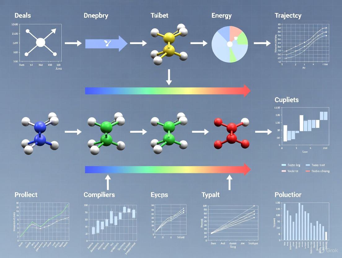
The following diagram illustrates a recommended workflow for tackling the common problems in MD trajectory analysis.

MD Trajectory Cleanup Workflow

Experimental Protocols & Data

Protocol 1: Full Trajectory Cleanup Pipeline using CPPTRAJ

This protocol combines steps to fix PBC, remove solvent, and align the trajectory [1].

• Input: Raw trajectory file (simulation.nc) and topology file (system.prmtop).
• Center the Protein: Center the primary protein domain in the box.

• Unwrap Other Molecules: Ensure ligands or other domains stay connected to the protein.

• Run Autoimage: Rebuild the simulation box around the centered and unwrapped molecules.

• Strip Solvent: Remove water and ions to drastically reduce system size.

• Align Trajectory: Remove overall rotation and translation by fitting to the backbone.

• Output: Save the final, cleaned trajectory.

Protocol 2: Quantifying the Impact of Trajectory Compression

This protocol outlines how to compress a trajectory and evaluate the effect on energy calculations, based on findings from quantitative studies [4].

• Compress Trajectory: Convert your trajectory to a NetCDF4/HDF5 format with quantization (e.g., using CPPTRAJ). The quantization level (e.g., 100x) determines the precision loss [4].
• Calculate Energies: Perform energy calculations (e.g., MM-PB/GB-SA) on both the original and compressed trajectories.
• Quantify Error: Calculate the Root Mean Square Error (RMSE) for the total energy and individual terms (Electrostatics, VdW, Bonds, Angles) between the two datasets [4].
• Analyze Trade-offs: Evaluate if the achieved compression ratio is worth the introduced energy error for your specific analysis goals. A quantization of 100x often offers a good compromise [4].

Quantitative Data on Trajectory Compression

The table below summarizes how different compression methods affect coordinate precision and subsequent energy calculations, based on research data [4].

Format / Method	Coordinate Precision	Avg. Position RMSD (Å)	Energy RMSE (kcal/mol)	Key Consideration
NetCDF4 (i1.nc4)	1x (0.1 Å)	~0.1	Can be >1	Significant energy error, not recommended.
NetCDF4 (i3.nc4)	1000x (0.001 Å)	~0.001	Low (~0.001)	Good for most analyses, similar to ASCII .crd.
GROMACS XTC	3 decimals (in nm)	~0.01	Low	Good compression, standard in GROMACS.
Amber ASCII (.crd)	3 decimals (in Å)	~0.001	Low (but VdW higher)	Very large file size, not efficient.

Note: The flexible bond energy term is particularly sensitive to compression and shows higher errors for non-constrained water models [4].

Navigating Periodic Boundary Condition (PBC) Artifacts in Biomolecular Visualizations

FAQs: Understanding PBC Artifacts

Q1: Why do my molecules appear broken or have bonds extending across the simulation box? This is a classic visualization artifact, not an error in the simulation dynamics. Under Periodic Boundary Conditions (PBC), the simulation box is surrounded by translated copies of itself. When a molecule crosses the boundary of the primary box, it is "broken" as one part exits (e.g., on the right) and simultaneously re-enters from the opposite side (e.g., on the left). Visualization software often renders this as a long bond across the entire box [6]. The molecule itself remains chemically intact.

Q2: What causes sudden "jumps" in measured distances between atoms over time? These jumps occur because standard trajectory analysis might track coordinates without accounting for PBC. When a molecule crosses the box boundary, its coordinates can discontinuously jump from one side of the box to the other. The measured distance between this molecule and a stationary reference point will then show a sudden, large change, even though the actual physical separation has changed only minimally [7].

Q3: How does the shape and size of the periodic box influence artifacts? The box size and shape are critical factors [8] [9].

• Size: A box that is too small can cause a macromolecule to artificially interact with its own periodic image. A common recommendation is to have at least 1.0 nm of solvent between the solute and the box edge [10] [8].
• Shape: A cubic box is simple but inefficient, containing solvent in corners far from the solute. For globular molecules, a rhombic dodecahedron or truncated octahedron is often more efficient as it more closely approximates a sphere, requiring ~29% fewer solvent molecules for the same minimum image distance [8] [9].

Q4: What are the system-level requirements for PBC to function correctly? Two key restrictions must be met [9]:

• Charge Neutrality: The net electrostatic charge of the entire system must be zero to avoid infinite energy sums when PBC are applied. This is typically achieved by adding counterions [10].
• Cut-off Criterion: The cut-off radius (Rc) for short-range non-bonded interactions must be less than half the length of the shortest box vector: Rc < ½ min(||a||, ||b||, ||c||). This ensures a particle only interacts with the closest image of any other particle [9].

Troubleshooting Guide: Resolving Common Visualization Issues

Issue 1: Broken Molecules and Unphysical Bonds

Problem: During visualization, molecules are split across the box with long, seemingly unphysical bonds stretching from one side to the other [6].

Solution: Use the trjconv utility in GROMACS to make molecules "whole" again.

• Protocol:

• Mechanism: The -pbc mol flag identifies all molecules in the system and reassembles each one completely within the primary simulation box, removing the visual artifact of bonds crossing the periodic boundary [6].

Issue 2: Jumps in Trajectories and Distance Measurements

Problem: Analysis of atomic distances over time shows discontinuous jumps, complicating the study of continuous diffusion or conformational changes [7].

Solution: Remove these jumps from the trajectory before analysis.

• Protocol:

• Mechanism: The -pbc nojump algorithm checks the periodic image of each particle relative to its position in the reference structure and adjusts coordinates to avoid discontinuous jumps across the box, resulting in a continuous trajectory [7] [6].

Issue 3: System is Not Centered for Visualization

Problem: The molecule or complex of interest drifts from the center of the box, making visualization and filming difficult.

Solution: Center the system on your molecule of interest.

• Protocol:

• Mechanism: When prompted, select the group (e.g., "Protein") you wish to center in the box. The command shifts the entire system so that the center of mass of the selected group is placed at the center of the box [6].

Comprehensive Visualization Workflow

For a clean, publication-ready visualization, a specific sequence of trjconv commands is recommended. The diagram below illustrates this workflow.

Table 1: Key Software Tools for Managing PBC and Trajectory Analysis.

Tool Name	Primary Function	Relevance to PBC Artifacts
GROMACS (trjconv)	Molecular dynamics simulation and trajectory processing	The primary tool for correcting PBC-related visualization issues, including making molecules whole, removing jumps, and centering [7] [6].
MDTraj	Python library for MD trajectory analysis	A modern library that can read and write trajectory data in multiple formats and includes functions for handling PBC during analysis, such as RMSD calculations [11].
VMD / PyMOL	Molecular visualization	Industry-standard visualization software. Correcting trajectories with tools like trjconv before loading them into these programs is essential for accurate visual interpretation [12].
Particle Mesh Ewald (PME)	Algorithm for long-range electrostatics	A method used during the simulation itself to handle electrostatic interactions in a periodic system, mitigating artifacts from the artificial truncation of these forces [9] [13].

Advanced Considerations and Recent Research

Quantitative Impact of System Size

Recent research systematically investigates how the simulated system's size influences properties under PBC. The table below summarizes key findings from a 2024 study on peptide membranes [13].

Table 2: Effects of Increasing Simulation Box Size on Membrane Properties [13].

Property Measured	Small System (Under PBC Influence)	Large System (PBC-Free Core)	Change
Hydrogen Bond Lifetime	Baseline	~19% Increase	Significant increase, indicating small boxes may artificially stabilize interactions [13].
Amino Acid Dihedral Angle Mobility	Restricted	Higher	Greater conformational freedom in larger systems free from PBC constraints [13].
Property Convergence (e.g., Area per Molecule)	Non-convergent	Convergent	Macroscopic properties only reach stable values in sufficiently large systems [13].

Best Practices for Minimizing PBC Artifacts in Research

• Validate Box Size: Do not use a box that is merely "large enough" to hold the solute. Ensure the shortest box vector is at least twice the non-bonded cut-off radius [9]. For macromolecules, maintain a minimum of 1.0 nm of solvent padding in all directions [10] [8].
• Choose an Optimal Box Shape: For a globular protein in solution, a rhombic dodecahedron is highly recommended as it minimizes the number of solvent atoms needed while maintaining the required distance to periodic images, significantly improving computational efficiency [8] [9].
• Pre-process Trajectories for Analysis: Never analyze raw trajectories for properties like diffusion, distance, or RMSD. Always apply appropriate PBC corrections first to ensure data continuity and validity [11] [6].
• Be Aware of Advanced Artifacts: Understand that PBC can suppress long-wavelength fluctuations (e.g., in membranes) [13], influence bulk properties like system dipole moments [10], and conserve linear momentum but not angular momentum [10].

Managing Structural Drift and Ensemble Variability in Protein Simulations

Troubleshooting Guides

FAQ 1: Why does my protein simulation look exploded when I load it into visualization software?

Problem: Your protein complex appears fragmented, with domains scattered across the simulation box or pieces seemingly teleported to opposite sides.

Root Cause: This visual chaos is primarily caused by Periodic Boundary Conditions (PBC), a computational method that simulates bulk environment by treating the simulation box as a repeating tile. When molecules cross the box boundaries, they reappear on the opposite side. While physically correct for the simulation, this creates visualization artifacts because different parts of the protein cross boundaries at different times [1].

Solution: The solution involves "re-imaging" the trajectory to place all molecules back into the primary simulation box relative to a fixed anchor point, typically your main protein domain.

Protocol 1: Fixing PBC Artifacts with CPPTRAJ

Protocol 2: Fixing PBC Artifacts with MDAnalysis in Python

Problem: Your entire protein complex tumbles and translates through space during simulation, making meaningful analysis of internal motions and distance measurements impossible.

Root Cause: Structural drift occurs as proteins naturally diffuse and rotate in solution. Without alignment, this overall motion contaminates measurements of internal conformational changes [1].

Solution: Perform least-squares fitting of each trajectory frame to a reference structure (usually the first frame or an average structure) to remove overall translation and rotation.

Protocol: Structural Alignment with CPPTRAJ

Quantitative Assessment of Structural Drift: After alignment, quantify residual structural changes using Root-Mean-Square Deviation (RMSD):

FAQ 3: How can I efficiently analyze conformational heterogeneity from my simulation ensemble?

Problem: You need to identify and characterize the distinct conformational states sampled during your simulation and understand transitions between them.

Root Cause: Proteins exist as dynamic ensembles of interconverting structures rather than single static conformations. Analyzing this heterogeneity requires specialized approaches beyond simple averaging [14] [15] [16].

Solution: Employ dimensionality reduction and clustering techniques to identify metastable states and quantify transitions between them.

Protocol: Conformational State Analysis with EnsembleFlex

EnsembleFlex provides a comprehensive suite for analyzing conformational heterogeneity:

Advanced Protocol: Markov State Model Analysis

For more sophisticated ensemble analysis, Markov State Models (MSMs) can identify kinetic states and transition rates:

Workflow Diagram

Research Reagent Solutions

Table 1: Essential Software Tools for Managing Structural Drift and Ensemble Variability

Tool Name	Primary Function	Key Features	Application Context
CPPTRAJ [1]	Trajectory processing & analysis	PBC correction, structural alignment, RMSD calculation, solvent stripping	AMBER ecosystem; comprehensive trajectory preprocessing
MDAnalysis [1]	Python trajectory analysis	PBC handling, transformation pipeline, interoperability with Python data science stack	Custom analysis workflows, integration with machine learning libraries
EnsembleFlex [15]	Ensemble analysis	Dual-scale flexibility analysis, dimensionality reduction, binding site mapping, conserved water detection	Conformational heterogeneity analysis, drug design applications
MDTraj [11]	Molecular dynamics trajectory analysis	Fast RMSD calculations, secondary structure assignment, order parameter extraction	Lightweight, efficient analysis with Python integration
SAMSON [17]	Structure validation & preparation	Alternate location resolution, steric clash detection, rotamer editing	Pre-simulation structure validation and cleanup

Key Quantitative Metrics for Ensemble Variability

Table 2: Essential Metrics for Quantifying Structural Drift and Ensemble Variability

Metric	Calculation Method	Interpretation	Threshold Guidelines
RMSD (Root-Mean-Square Deviation)	$$RMSD = \sqrt{\frac{1}{N}\sum{i=1}^{N} \deltai^2}$$	Measures global structural change from reference	<2Å: minimal drift; 2-4Å: expected flexibility; >4Å: possible unfolding
RMSF (Root-Mean-Square Fluctuation)	$$RMSF = \sqrt{\langle (ri - \langle ri \rangle)^2 \rangle}$$	Quantifies per-residue flexibility	High values indicate flexible loops/termini; low values indicate stable core
Principal Component (PC) Variance	Eigenvalue decomposition of covariance matrix	Identifies dominant collective motions	First 3-5 PCs typically capture >70% of significant motions
State Populations	Cluster analysis or MSM eigenanalysis	Proportion of simulation in each conformational state	Determines thermodynamic stability of states
Transition Rates	Markov State Model analysis	Kinetics of interconversion between states	Slow rates (μs-ms) indicate high energy barriers

• Always preserve original trajectories - processing steps are irreversible [1]
• Validate structures before simulation to prevent failures from structural issues [17]
• Remove solvent before analysis when focusing on protein dynamics to reduce file size and speed up computation [1]
• Use multiple metrics to characterize ensemble variability from complementary perspectives [15]
• Combine experimental and computational data when possible for more accurate ensemble generation [14]

FAQs on Data Handling and Analysis

Q1: What are the primary challenges when working with multi-terabyte Molecular Dynamics (MD) trajectory data? The key challenges involve the sheer volume and complexity of the data. Modern high-performance computing allows simulations of biologically large systems, generating trajectories with millions to billions of atoms over long timescales. This results in hundreds to thousands of individual trajectories, creating massive datasets that are difficult to store, process, and visualize. The complexity of these systems makes it challenging to scrutinize the trajectories and extract biologically significant information about structures and dynamics [12].

Q2: What are the best practices for ensuring robustness and reproducibility in my simulations? To ensure your simulations are robust and reproducible, you should follow hypothesis-driven approaches and use reliable tools and databases. Critical practices include maintaining detailed records of simulation parameters, using validated force fields, and ensuring proper data curation. Promoting reproducibility and accessibility through reliable databases is also a fundamental best practice [18].

Q3: How can I effectively visualize such large trajectory datasets? Effective visualization is a major challenge. Traditional frame-by-frame visualization is often insufficient. Consider these approaches:

• Advanced Visualization Tools: Utilize modern software that can leverage GPU acceleration for handling large datasets [12].
• Web-Based Tools: Use web-based visualization tools for easier access, collaboration, and sharing of simulations [12].
• Interactive Widgets: Employ notebook-like environments with interactive molecular visualization widgets to facilitate analysis [12].
• Novel Techniques: Explore new visualization techniques being developed specifically to handle the scale and complexity of modern MD data, including immersive virtual reality environments for a more intuitive exploration [12].

Q4: Can machine learning help in analyzing these large datasets? Yes, machine learning, particularly deep learning, is a powerful tool for analyzing high-dimensional MD data. It can be used to embed complex simulation data into a lower-dimensional latent space that retains essential molecular characteristics. This simplifies the analysis and allows for the development of surrogate models that can predict constitutive behavior and failure, significantly reducing the need for repetitive, costly simulations [19] [12].

Troubleshooting Common Experimental Issues

Issue 1: Inability to process all trajectories due to memory limitations.

• Problem: Loading multiple multi-gigabyte trajectory files for analysis crashes the software or exhausts server RAM.
• Solution:
  • Implement Data Chunking: Use analysis tools that can read and process the trajectory in segments rather than loading it entirely into memory.
  • Leverage Stochastic Sampling: If studying a stochastic process, analyze multiple smaller, randomized subsets of frames to estimate the overall system behavior. This provides a statistically valid result without processing every frame.
  • Use Optimized Software: Employ specialized trajectory analysis packages designed for high-throughput data handling.

Issue 2: Difficulty in quantifying dispersion and identifying dominant motion paths in a cluster of trajectories.

• Problem: Visual inspection of hundreds of overlapping trajectories is overwhelming, making it impossible to quantify the common path and variance.
• Solution: Apply probabilistic trajectory modeling tools. These tools model the ensemble of trajectories as a Gaussian process, which provides a statistical summary. The output includes a mean path (the average trajectory) and a confidence region (a volume showing where a certain percentage of trajectories travel), thereby quantifying dispersion and identifying dominant motion patterns [20].

Issue 3: Long simulation times are a bottleneck for exploring different conditions.

• Problem: Running full MD simulations for every parameter variation or initial condition is computationally prohibitive.
• Solution: Develop a machine learning-based surrogate model (metamodel). Train a model, such as a Gated Recurrent Unit (GRU) neural network, on existing MD simulation data. Once trained, this model can almost instantaneously predict the constitutive response and failure of the material under unseen loading patterns, bypassing the need for new, full-scale simulations [19].

Issue 4: Choosing an inappropriate data visualization for communicating results.

• Problem: The selected chart type leads to misinterpretation of the hierarchical or comparative data.
• Solution: Match the visualization to the data type and communication goal.
  • For Hierarchical Data: Treemaps can show part-to-whole relationships for large, hierarchical data, but they are hard to use for precise comparisons. Use them with caution, ensuring high-level categories have visually distinct borders [21].
  • For Comparisons: Sorted bar charts are often preferable for comparing the values of different items, as the human brain can pre-attentively process length comparisons more accurately than area [21].
  • For Relationships: Scatter plots are excellent for showing the relationship between two numeric variables [22].

Data Presentation: Comparison of Storage Solutions

The table below summarizes key quantitative aspects of different storage formats and strategies for managing large trajectory data.

Table 1: Comparison of Trajectory Data Storage and Analysis Formats

Format / Strategy	Typical Size Reduction	Read Speed	Write Speed	Best Use Case
Uncompressed Trajectory	Baseline	Very Fast	Very Fast	Short-term, active analysis
Lossless Compression (e.g., XTC)	~50-80%	Fast	Fast	Long-term storage, full-fidelity analysis
Lossy Compression	~90-99%	Fast	Medium	Remote visualization, initial exploratory analysis
Feature-Reduced Data (e.g., order parameters)	~99%+	Very Fast	Slow	Machine learning training, specific property analysis
Surrogate ML Model	>99.9% (after training)	Instant (post-inference)	Very Slow (training)	Rapid prediction and scenario testing [19]

Experimental Protocol: Creating an ML-Based Surrogate Model

This protocol outlines the methodology for developing a machine learning surrogate to replace full MD simulations, based on the approach cited in the research [19].

Objective: To create a trained neural network model that can predict the rate-dependent and path-dependent constitutive and damage behavior of a composite material, bypassing the need for full MD simulations.

Materials:

• Hardware: High-Performance Computing (HPC) cluster with GPUs.
• Software: MD simulation package (e.g., GROMACS, LAMMPS), Python with deep learning libraries (TensorFlow/PyTorch), and data processing libraries (NumPy, Pandas).

Methodology:

• Data Generation via MD:
  • Model Constituents: Run separate MD simulations for each constituent material (e.g., epoxy matrix, glass fiber) and their interface.
  • Systematic Loading: Apply a diverse set of strain paths and loading rates to each model to cover a wide spectrum of mechanical responses.
  • Data Extraction: For each simulation, extract the stress tensor and a damage indicator (e.g., void fraction, number of broken bonds) at each time step. The time step information must be embedded with the strain path data.

• Data Curation and Preprocessing:

  • Aggregation: Compile the stress, damage, and corresponding strain-time data from all simulations into a unified dataset.
  • Normalization: Normalize all input (strain, time) and output (stress, damage) variables to a common scale (e.g., 0 to 1) to ensure stable and efficient model training.
  • Partitioning: Split the dataset into training (∼70%), validation (∼15%), and testing (∼15%) subsets.

• Model Training and Validation:

  • Architecture: Construct a multi-task Gated Recurrent Unit (GRU)-based neural network. The GRU layers are designed to capture path-dependent and rate-dependent temporal evolution.
  • Multi-Task Output: Configure the network with two output heads: one for predicting the stress tensor and another for predicting the damage indicator.
  • Training Loop: Train the model on the training set, using the validation set for hyperparameter tuning and to prevent overfitting. The loss function should combine the mean squared error for stress and the cross-entropy loss for damage.
  • Testing: Evaluate the final model's performance on the unseen test set by comparing its predictions against the ground-truth MD simulation results.

The Scientist's Toolkit: Essential Research Reagents & Software

Table 2: Key Software and Analytical Tools for MD Trajectory Analysis

Tool Name	Function	Application Note
GROMACS/LAMMPS	High-performance MD simulation engines	Used for generating the initial multi-terabyte trajectory data.
Teetool	Python package for probabilistic trajectory analysis	Models trajectories as a Gaussian process to visualize confidence regions and quantify dispersion [20].
GRU-based Neural Network	Deep learning model for sequential data	Serves as the core architecture for the surrogate model, capturing rate- and path-dependent material behavior [19].
Web-Based Visualization Tools (e.g., Mol* Viewer)	Accessible platforms for viewing and sharing trajectories	Facilitates collaboration and provides an intuitive interface for inspecting structural dynamics without local installation of heavy software [12].
Jupyter Notebooks	Interactive computing environment	Ideal for integrating analysis scripts (e.g., with Teetool), data visualization widgets, and documentation into a single, reproducible workflow [20].

Workflow Visualization

The following diagram illustrates the integrated strategy for handling multi-terabyte trajectory datasets, from data generation to insight delivery.

Frequently Asked Questions (FAQs)

1. What do sudden jumps in my RMSD plot indicate, and how can I resolve them? Sudden jumps in RMSD often result from periodic boundary condition (PBC) artifacts, not true structural changes. Your protein may be moving across the simulation box, causing coordinates to "wrap" and misalign when visualized or analyzed [1].

• Solution: Process your trajectory to remove PBC artifacts before analysis. Use tools like CPPTRAJ or MDAnalysis to center your protein in the box and "unwrap" the coordinates so the molecule remains intact across periodic images [1].

2. My Radius of Gyration (Rg) suggests protein unfolding, but the structure looks native. What should I check? A rising Rg can indicate expansion or unfolding [23]. First, visually inspect multiple trajectory frames to confirm global structural changes versus local fluctuations. Then, cross-validate with other metrics:

• Check SASA: An increasing SASA corroborates unfolding as the protein interior becomes solvent-exposed [24].
• Check RMSD: Rising RMSD suggests a global conformational shift from the native state [25].
• Check Intra-protein H-bonds: A significant decrease in intramolecular hydrogen bonds supports loss of compact structure [24].

3. How do I interpret conflicting stability signals from SASA and Rg? Rg and SASA typically correlate, measuring overall compactness and solvent exposure. Conflict may arise from localized changes:

• Scenario: Rg is stable, but SASA increases.
• Interpretation: The protein's overall dimensions remain stable, but surface residues may be undergoing rearrangement, creating new pockets or crevices without major expansion.
• Action: Perform per-residue SASA analysis or inspect structural snapshots to identify localized surface changes.

4. Why is my protein-ligand interaction energy favorable, but the ligand dissociates? Favorable average interaction energy can be misleading if the ligand samples both bound and unbound states during simulation.

• Diagnosis: Plot the ligand's center of mass (COM) distance from the binding pocket over time. A increasing distance confirms dissociation [26].
• Root Cause: The simulation may have captured a genuine dissociation event, or the initial pose was unstable. Check if the ligand RMSD relative to the protein is stable before dissociation [26].

5. How can I ensure my RMSD analysis is meaningful? A drifting RMSD can indicate structural drift, but it must be analyzed relative to a correct reference and with proper alignment.

• Proper Workflow:
  • Remove PBC effects to ensure the protein is whole and coordinates are continuous [1].
  • Align all frames to a reference structure (e.g., the initial protein backbone or a stable domain) to remove overall rotation and translation [1].
  • Calculate RMSD for the protein backbone or specific domains of interest [26].

Metric Interpretation and Troubleshooting Guide

The table below summarizes the fundamental metrics, their structural significance, and common issues encountered during analysis.

Metric	Primary Structural Insight	Typical Output for a Stable, Folded Protein	Common Calculation Pitfalls & Fixes
Root Mean Square Deviation (RMSD) [25] [26]	Measures the average change in atom positions relative to a reference structure over time; quantifies global conformational stability.	Reaches a stable plateau after an initial equilibration period.	Pitfall: Noisy or continuously rising RMSD.Fix: Ensure trajectories are centered and aligned to a reference (e.g., backbone atoms) after fixing PBC issues [1].
Radius of Gyration (Rg) [23] [26]	Measures the overall compactness and density of the protein structure.	Maintains a stable, low value, indicating a tight, folded core.	Pitfall: Misleading Rg values due to protein tumbling or PBC artifacts.Fix: Use a centered and aligned trajectory. A rising Rg should be correlated with SASA and visual inspection [23] [1].
Solvent Accessible Surface Area (SASA) [24] [26]	Quantifies the surface area of the protein accessible to a solvent molecule; indicates packing efficiency and exposure of hydrophobic cores.	Remains relatively constant, with minor fluctuations.	Pitfall: SASA increases without a corresponding Rg increase.Fix: Analyze for local surface changes or pocket opening. Ensure the calculation uses a consistent solvent radius (typically 1.4 Å).
Interaction Energy [26]	Calculates the non-covalent interaction energy (electrostatic + van der Waals) between molecules, such as a protein and ligand.	Remains stably favorable (negative) for a specific, bound complex.	Pitfall: Favorable energy despite ligand dissociation.Fix: Always correlate with ligand RMSD and COM distance to confirm the bound pose is maintained throughout the simulation [26].

Essential Experimental Protocols

Protocol 1: Standard Workflow for MD Trajectory Analysis

This protocol outlines the critical steps for preparing a raw molecular dynamics trajectory for robust analysis of RMSD, Rg, SASA, and other metrics [1] [26].

Procedure:

• Fix Periodic Boundary Conditions (PBC): Use a tool like CPPTRAJ or MDAnalysis to center the protein in the simulation box and unwrap coordinates. This ensures the protein appears as a single, continuous molecule.
  • CPPTRAJ Command:
    [1]
• Strip Solvent: Remove water and ions to drastically reduce file size and speed up subsequent analysis.
  • CPPTRAJ Command:
    [1]
• Align Trajectory: Perform a least-squares fit of all trajectory frames to a reference structure (e.g., the initial protein backbone) to remove global rotation and translation. This is essential for meaningful RMSD calculations.
  • MDAnalysis Command:
    [1]
• Calculate Metrics: Perform the desired analyses on the cleaned trajectory.

Protocol 2: Assessing Protein Stability via RMSD, Rg, and SASA

This protocol describes how to jointly interpret key metrics to evaluate the stability of a protein or protein-ligand complex during a simulation [23] [25] [24].

Procedure:

• Run Simulation: Perform an all-atom molecular dynamics simulation for the desired timescale (e.g., 100 ns - 1 µs).
• Process Trajectory: Follow Protocol 1 to generate a clean, aligned trajectory.
• Calculate Time-Series Data:
  • RMSD: Calculate the backbone RMSD relative to the energy-minimized starting structure for every frame.
  • Rg: Compute the radius of gyration for the protein's Cα atoms for every frame.
  • SASA: Calculate the total solvent-accessible surface area for the protein for every frame.
• Correlate and Interpret:
  • A stable, folded protein will show RMSD, Rg, and SASA values that converge to a plateau after initial equilibration, with fluctuations around a stable average [25].
  • A destabilizing or unfolding event is characterized by a coordinated increase in RMSD, Rg, and SASA, indicating a loss of native structure and expansion of the protein [23] [24].
  • For protein-ligand complexes, calculate the same metrics for the protein alone and monitor ligand-specific metrics like ligand RMSD to assess binding stability [26].

Protocol 3: Calculating Protein-Ligand Interaction Energies

This protocol outlines the steps for determining non-covalent interaction energies, a key metric for quantifying binding affinity in complexes [26].

Procedure:

• Prepare the System: Ensure your topology and trajectory files include both the protein and the bound ligand.
• Define Interaction Groups: Specify the atom groups for the protein and the ligand.
• Calculate Energy Components: Use molecular mechanics to calculate the van der Waals and electrostatic interaction energies between the two groups for each trajectory frame. Many MD packages (e.g., GROMACS via gmx energy, SILCSBIO CGenFF Suite [26]) have built-in utilities for this.
• Analyze Time-Series: The total interaction energy is the sum of the two components. A stable, favorably bound complex will exhibit a consistently negative (favorable) total interaction energy throughout the simulation.
• Cross-Reference with Structural Data: Always correlate stable, favorable interaction energies with a stable ligand RMSD and a consistent protein-ligand binding pose to confirm the integrity of the complex.

The Scientist's Toolkit: Research Reagent Solutions

The table below lists essential software tools and their functions for molecular dynamics trajectory analysis.

Tool Name	Primary Function	Key Utility in Trajectory Analysis
GROMACS [27]	A versatile package for performing molecular dynamics simulations.	The primary engine for running simulations. Its suite of tools (gmx rms, gmx gyrate, gmx sasa, gmx energy) is used for calculating RMSD, Rg, SASA, and interaction energies, respectively.
CHAPERONg [27]	An automation tool for GROMACS-based simulation pipelines.	Automates the entire workflow of system setup, simulation run, and post-processing analysis, including the calculation of RMSD, Rg, and SASA, reducing manual intervention and potential for error.
CPPTRAJ [1]	The main analysis utility in the AmberTools package.	A powerful and versatile tool for processing and analyzing MD trajectories. Excels at fixing PBC issues, stripping solvent, aligning trajectories, and calculating a vast array of structural and dynamic metrics.
MDAnalysis [1]	A Python library for analyzing molecular dynamics trajectories.	Provides a programmable environment for trajectory analysis. Allows users to write custom Python scripts to load, manipulate (e.g., fix PBC, align), and analyze trajectories, offering high flexibility.
VMD [23]	A molecular visualization and analysis program.	Primarily used for visualizing trajectories to qualitatively confirm structural states, binding poses, and artifacts. It also contains built-in functions for various analyses.

Advanced Analysis Techniques for Drug Discovery Applications

Radial Distribution Functions (RDF) for Analyzing Solvation and Binding Sites

Radial Distribution Functions (RDF) are fundamental tools in molecular dynamics (MD) analysis for quantifying how particle density varies as a function of distance from a reference particle. The RDF (g_{ab}(r)) between types of particles (a) and (b) is defined as:

[g{ab}(r) = (N{a} N{b})^{-1} \sum{i=1}^{Na} \sum{j=1}^{Nb} \langle \delta(|\mathbf{r}i - \mathbf{r}_j| - r) \rangle]

This function normalizes to 1 for large separations in a homogenous system, effectively counting the average number of (b) neighbours in a shell at distance (r) around an (a) particle and representing it as a density [28]. In thesis research, RDF analysis provides critical insights into solvation shells, binding site identification, and molecular interaction patterns in drug development studies.

Implementing RDF Analysis: A Practical Guide

How do I calculate a basic Radial Distribution Function?

Solution: Use the InterRDF class in MDAnalysis for average RDFs between two groups of atoms.

This code calculates the average RDF between all atoms in the solute and solvent groups, providing insights into overall solvation structure [28].

What's the difference between InterRDF and InterRDF_s?

Solution: InterRDF calculates average RDFs between groups, while InterRDF_s provides site-specific RDFs for individual atom pairs.

Site-specific RDFs are crucial for understanding detailed interactions in binding pockets and specific solvation sites [28].

Troubleshooting Common RDF Analysis Issues

Why is my RDF plot too noisy or inconsistent?

Problem: Noisy RDF profiles often result from insufficient sampling or incorrect trajectory handling.

Solutions:

• Increase sampling: Ensure your analysis includes enough trajectory frames for statistical significance
• Check system stability: Verify that your simulation has properly equilibrated before analysis
• Adjust bin parameters: Increase the number of bins (nbins) for higher resolution or decrease if oversampled
• Validate trajectory loading: Confirm your Universe object properly loads all trajectory frames using print(len(u.trajectory))

How do I calculate coordination numbers from RDF data?

Problem: Researchers often need to extract quantitative coordination numbers from RDF profiles.

Solution: Use the cumulative distribution function available in MDAnalysis.

The position of the first minimum in (g(r)) typically defines the first solvation shell radius (r1), and (N(r1)) gives the coordination number [28].

How do I analyze specific molecular orientations in RDF calculations?

Problem: Standard RDF analysis doesn't account for molecular orientation effects.

Solution: Implement vector-based analysis for oriented systems, as demonstrated in dye-polymer systems:

This approach helps analyze how molecular orientation affects distribution functions in anisotropic systems [29].

Experimental Protocols and Methodologies

Protocol 1: Solvation Shell Analysis for Transition Metal Complexes

Application: Analyzing solvation shells of electrochemically active redox couples in aqueous solution [30].

Methodology:

• System Preparation: Run ab initio molecular dynamics using PBE functional with/without Tkatchenko-Scheffler van der Waals corrections
• Trajectory Analysis: Calculate RDFs between metal centers and solvent oxygen atoms
• Key Systems: Analyze Cr²⁺/³⁺, V²⁺/³⁺, Ru(NH₃)₆²⁺/³⁺, Sn²⁺/⁴⁺, Cu¹⁺/²⁺, ferrocene methanol, Fe²⁺/³⁺, and ferrocene
• Data Interpretation: Identify solvation shell boundaries from RDF minima and calculate coordination numbers

Expected Results: Distinct solvation shells with different coordination numbers for various oxidation states, providing insights into solvation structure changes during redox processes.

Protocol 2: Binding Site Analysis for Drug Discovery

Application: Characterizing ligand binding sites and interaction patterns in protein-ligand systems.

Methodology:

• Trajectory Preparation: Run MD simulation of protein-ligand complex in explicit solvent
• Site Identification: Select key binding site residues and ligand atoms
• Site-Specific RDF: Use InterRDF_s to calculate pairwise RDFs between binding site atoms and ligand atoms
• Residence Time Analysis: Calculate survival probabilities for solvent molecules in binding site
• Competitive Binding Assessment: Analyze RDFs between binding site and water/co-solvent molecules

Interpretation: Sharp, high peaks in site-specific RDFs indicate strong, specific interactions, while broad peaks suggest transient or weak interactions.

RDF Analysis Workflow Visualization

RDF Analysis Workflow

Key Parameters for RDF Analysis

Table 1: Critical RDF Calculation Parameters and Their Effects

Parameter	Default Value	Effect on Results	Recommendation
nbins	75	Higher values increase resolution but may introduce noise	Adjust based on system size (75-150)
range	(0.0, 15.0)	Defines distance range for analysis	Set maximum to half box size to avoid PBC artifacts
exclusion_block	None	Excludes bonded neighbors from same molecule	Use (n, n) for molecules with n atoms each
density	False	When True, returns true density (n{ab}(r)) instead of (g{ab}(r))	Use False for standard RDF, True for coordination numbers

Table 2: Common RDF Analysis Issues and Solutions

Problem	Possible Causes	Solutions
Noisy RDF	Insufficient sampling, small bin size	Increase trajectory frames, adjust nbins
Unphysical peaks	PBC artifacts, incorrect atom selection	Check PBC handling, validate atom groups
Flat RDF	Incorrect group selection, system not equilibrated	Verify group definitions, check equilibration
Memory errors	Large systems, too many frames	Use step parameter in run(), analyze subsets

The Scientist's Toolkit: Essential Research Reagents and Software

Table 3: Essential Tools for RDF Analysis in Molecular Dynamics

Tool/Resource	Function	Application Context
MDAnalysis	Python toolkit for MD trajectory analysis	Loading trajectories, RDF calculation, custom analysis [31]
InterRDF class	Calculates average RDF between atom groups	General solvation structure analysis [28]
InterRDF_s class	Calculates site-specific RDFs	Binding site analysis, specific interaction studies [28]
GROMACS	MD simulation package	Trajectory generation, system preparation [32]
BioExcel Building Blocks	Workflow library for MD setup and run	Streamlined simulation setup and analysis [32]

Advanced RDF Applications and Methodologies

How do I interpret RDFs for ionic liquid systems?

Context: Analysis of imidazolium-based ionic liquids in ethylene glycol requires special consideration of cation-anion and ion-solvent interactions [33].

Interpretation Guide:

• First peak position: Indicates contact ion pair distance
• Peak height: Reflects interaction strength and specificity
• Second shell structure: Reveals medium-range ordering and solvation patterns
• Chain length effects: Longer alkyl chains (C4mim+, C6mim+) show solvophobic solvation and structure-making tendencies [33]

Methodology:

• Combine RDF analysis with volumetric properties and conductivity measurements
• Calculate ion association constants from coordination number analysis
• Use molecular dynamics simulations to complement experimental RDF data

How do I validate RDF results for publication?

Quality Control Checklist:

• Verify statistical convergence by comparing RDFs from trajectory subsets
• Check for PBC artifacts by ensuring no peaks beyond half box length
• Validate atom selections by visualizing representative frames
• Confirm appropriate normalization by checking RDF approaches 1 at large r
• Compare with known experimental data where available
• Report all parameters (nbins, range, exclusion_block) in methods section

Integration with Broader Thesis Research

For comprehensive molecular dynamics trajectory analysis in thesis research, RDF analysis should be integrated with:

• Structural analysis: RMSD, RMSF, and radius of gyration calculations
• Energetic analysis: Binding free energy calculations
• Dynamical analysis: Hydrogen bond lifetimes, diffusion constants
• Experimental validation: Comparison with experimental spectroscopy data

This integrated approach provides a complete picture of molecular behavior in solution and binding environments, supporting robust conclusions in drug development research.

Calculating Binding Free Energies Using MM/PBSA and Umbrella Sampling

Frequently Asked Questions (FAQs)

MM/PBSA Methodology

Q1: My MM/PBSA results are unstable and vary significantly between short simulation replicates. What is the likely cause and how can I address this?

A: The likely cause is insufficient sampling. Short molecular dynamics (MD) simulations may give the illusion of convergence but often fail to capture slow conformational transitions that critically affect computed free energies.

• Problem Identification: If repeated short simulations (e.g., 5-10 ns) of the same system yield binding free energies with variations much larger than the expected chemical accuracy (1 kcal/mol), it indicates the underlying conformational ensemble has not been adequately sampled [34].
• Solution: Perform longer simulations or employ enhanced sampling techniques. Statistically, sampling sufficiency is a prerequisite for obtaining reliable results. Do not equate long simulation times with sufficient sampling; instead, use convergence analyses to determine if your simulation time covers the relevant conformational space. Adaptive sampling strategies can help balance efficiency and reliability [34].

Q2: How should I adapt the MM/PBSA protocol for membrane protein-ligand systems?

A: Standard MM/PBSA protocols, designed for soluble proteins, often fail for membrane systems due to the heterogeneous dielectric environment of the lipid bilayer. Key adaptations include [35]:

• Membrane-aware Dielectric Modeling: The continuum solvent model must account for the low-dielectric membrane region. Use tools like APBSmem or the updated MMPBSA.py in Amber, which provide automated options for calculating membrane placement parameters (thickness, center) directly from the trajectory, ensuring a consistent and physically realistic dielectric environment for the calculation [35].
• Multi-Trajectory Approach: For systems with large ligand-induced conformational changes, a single trajectory might be insufficient. Instead, use a multi-trajectory approach where separate simulations are performed for the unbound protein (e.g., in the apo state) and the protein-ligand complex. This prevents the forcing of an unrealistic conformation in the unbound state [35].
• Entropy Corrections: Incorporate entropy estimates, such as those from Truncated Normal Mode Analysis (NMA), which can be particularly important for capturing the thermodynamic impact of conformational changes in membrane proteins [35].

Q3: The entropic term (-TΔS) in MM/PBSA is computationally expensive and noisy. When is it necessary to include it?

A: The entropic contribution is often small compared to the large, opposing enthalpic and solvation terms. However, it can be critical for achieving accuracy in certain scenarios [36].

• You can often omit it when performing high-throughput ranking of congeneric ligands (very similar compounds), as the relative differences in entropy might be consistent and the ranking is driven by the enthalpy/solvation terms.
• You should include it when calculating absolute binding affinities, when comparing ligands that bind with significantly different modes (e.g., one induces a large conformational change while another does not), or when striving for the highest possible quantitative accuracy. For these cases, methods like normal-mode or quasi-harmonic analysis are used, though they are computationally demanding [36].

Umbrella Sampling Methodology

Q4: How can I objectively determine a good reaction coordinate (RC) for Umbrella Sampling without prior knowledge of the end state?

A: Manually selecting an RC is a major source of error. Automated approaches can now determine effective RCs directly from simulation data [37].

• Protocol: Initiate a non-equilibrated MD simulation from the known native state basin. From this trajectory, use statistical analysis tools, such as time-lagged independent component analysis, to identify the slowest collective degrees of freedom. These can serve as excellent RCs. This is the core idea behind tools like AutoSIM, which automates this process to generate free energy surfaces for functional conformational transitions without requiring a priori information on the RC or the final state [37].

Q5: How can I assess and improve the convergence of my Umbrella Sampling simulation?

A: Convergence must be statistically evaluated, not assumed from simulation length [37].

• Convergence Assessment: A robust method is to combine statistics from multiple independent Umbrella Sampling runs. By comparing the free energy profiles from these replicates, you can quantify statistical uncertainty. If the profiles differ significantly, convergence has not been achieved.
• Improving Convergence: If simulations are not converged, systematically increase the sampling within each umbrella window. Furthermore, the automated protocol in AutoSIM allows for combining statistics from multiple runs to systematically assess and improve the quality of the free energy projection along a chosen RC [37].

Troubleshooting Common Problems

MM/PBSA Troubleshooting

Problem	Possible Causes	Diagnostic Steps	Solutions
Unphysical or wildly fluctuating results	1. Severe undersampling [34].2. Incorrect system setup (e.g., bad contacts, incorrect protonation).3. Numerical instability in PB solver.	1. Check for convergence by dividing the trajectory into halves and comparing results [34].2. Visually inspect multiple trajectory frames for stability.3. Check energy logs for crashes.	1. Extend simulation time or use enhanced sampling [34].2. Re-run system minimization and equilibration.3. Adjust PB grid parameters (density, cutoff).
Poor correlation with experimental data	1. Force field inaccuracies [34].2. Lack of conformational sampling [34].3. Missing entropic term [36].4. Ignored key ligand/protonation states.	1. Verify force field compatibility with your ligand.2. Check if simulations sampled all relevant rotamers/poses.3. Test the impact of including -TΔS.	1. Use a different/validated force field or charge model.2. Use longer or replica-exchange simulations.3. Include entropic correction for final calculation.4. Test multiple ligand tautomers/protonation states.
High computational cost per snapshot	1. Large system size.2. Fine PB grid settings.3. Entropy calculation.	1. Profile the time taken by different calculation parts.	1. Use the Generalized Born (GB) approximation for initial screening.2. Use a distance-dependent dielectric for initial tests.3. Increase the time between analyzed snapshots.

Umbrella Sampling Troubleshooting

Problem	Possible Causes	Diagnostic Steps	Solutions
Poor overlap between umbrella windows	1. Windows are too far apart along the RC.2. The force constant for the harmonic bias is too weak.3. The RC is poorly chosen and couples multiple pathways.	1. Plot the probability distribution of the RC for each window.2. Check the histogram of collected data in each window.	1. Decrease the spacing between windows.2. Increase the harmonic force constant.3. Re-evaluate the choice of RC; consider a 2D PMF.
Free energy profile not converging	1. Inadequate sampling within windows [34].2. Slow degrees of freedom orthogonal to the RC are not sampled.	1. Perform block analysis (e.g., with WHAM) to see how the PMF changes with increasing simulation time.2. Check for collective motions not captured by the RC.	1. Extend sampling in each window, especially in transition state regions [37].2. Use an additional CV in a 2D US simulation or employ replica-exchange US.
High energy barriers that are rarely crossed	1. The RC does not correspond to the natural reaction pathway.2. The underlying atomistic energy landscape has a genuine high barrier.	1. Monitor if the system explores the entire RC range as expected.	1. Use automated tools (e.g., AutoSIM) to find a better RC [37].2. Apply a secondary bias along an orthogonal CV or use metadynamics.

The Scientist's Toolkit: Essential Research Reagents & Software

Table: Key Computational Tools for Binding Free Energy Calculations

Tool Name	Type/Category	Primary Function	Application Note
GROMACS [38]	MD Simulation Software	High-performance MD engine for running simulations.	Often used for producing the trajectories later analyzed by MM/PBSA or Umbrella Sampling.
AMBER [35]	MD Simulation & Analysis Suite	Includes MMPBSA.py for end-state free energy calculations.	The recent Amber24 update includes automated membrane parameters for MMPBSA calculations on membrane proteins [35].
AutoSIM [37]	Automated Sampling Algorithm	Redesigns and automates Umbrella Sampling.	Automatically determines reaction coordinates and assesses convergence, addressing key US limitations [37].
MDAnalysis [39]	Trajectory Analysis Library	Python library for analyzing MD trajectories.	Extensible toolset for in-depth analysis, including RMSD, SASA, and distance calculations; supports streaming analysis.
ProLIF [39]	Interaction Analysis Tool	Identifies protein-ligand interactions from MD trajectories.	Useful for complementing MM/PBSA by providing a residue-level interaction fingerprint to explain affinity differences.

Experimental Protocols & Workflows

Detailed Protocol: MM/PBSA for a Standard Protein-Ligand Complex

This protocol outlines the steps for performing an MM/PBSA calculation on a solvated protein-ligand complex using a single MD trajectory.

Step 1: System Preparation and Equilibration

• Parameterize the Ligand: Use the antechamber program (from AmberTools) with the GAFF force field and AM1-BCC charges to generate topology and coordinate files for the ligand.
• Assemble the Complex: Combine the protein (with a standard force field like ff19SB) and ligand parameter files to create the complex. Solvate the complex in a TIP3P water box, ensuring a minimum buffer distance (e.g., 12 Å). Add ions to neutralize the system's charge and achieve a physiological salt concentration (e.g., 150 mM NaCl).
• Energy Minimization: Perform 5000 steps of steepest descent minimization to remove bad contacts.
• System Heating: Gradually heat the system from 0 K to 300 K over 100 ps under an NVT ensemble with positional restraints (e.g., 5 kcal/mol/Ų) on the protein and ligand heavy atoms.
• System Equilibration: Perform at least 1 ns of NPT simulation at 300 K and 1 bar, gradually releasing the positional restraints. Monitor the density and potential energy for stability.

Step 2: Production MD Simulation

• Run an NPT production simulation. The length should be determined by convergence testing, but a common starting point is 100-200 ns. Save trajectory frames every 100 ps for subsequent analysis. The stability of the system should be confirmed by analyzing metrics like the root-mean-square deviation (RMSD) of the protein backbone and ligand [34].

Step 3: MM/PBSA Calculation

• Extract snapshots from the equilibrated portion of the trajectory (e.g., every 1 ns) for the MM/PBSA calculation. A typical approach uses 500-1000 snapshots.
• Use the MMPBSA.py script from AmberTools. An example command is:

• A sample input file (mmppbsa.in) would contain:

Detailed Protocol: Umbrella Sampling for a Conformational Transition

This protocol describes how to use Umbrella Sampling to calculate the free energy profile (PMF) for a biomolecular conformational transition.

Step 1: Determine the Reaction Coordinate (RC) and Generate Initial Structures

• RC Selection: If the end states are known (e.g., open and closed form of a protein), a simple RC could be the distance between two key Cα atoms or the radius of gyration. For unknown pathways, use an automated tool like AutoSIM to determine the RC from an unbiased MD simulation [37].
• Steered MD (SMD): Perform a SMD simulation to rapidly pull the system from one end state (A) to the other (B) along the chosen RC. This generates a starting path.

Step 2: Set Up Umbrella Sampling Windows

• Extract multiple snapshots (e.g., 20-50) from the SMD trajectory at regular intervals along the RC. These will serve as the initial configurations for each umbrella window.
• For each window, set up an independent simulation with a harmonic biasing potential, ( U{\text{bias}} = \frac{1}{2} k (ξ - ξi)^2 ), where ( k ) is the force constant and ( ξ_i ) is the center of the RC for the i-th window. The force constant should be strong enough to ensure good overlap between adjacent windows but not so strong as to restrict sampling within the window.

Step 3: Run Equilibrated Simulations and Check Overlap

• Run an equilibrated MD simulation for each window. The simulation length must be sufficient to sample the local conformational space. Monitor the RC value in each window to ensure it fluctuates around its center.
• After simulations, check the overlap of the RC distributions between adjacent windows. If there are gaps, you may need to add more windows or increase sampling in existing ones.

Step 4: Analyze Data and Construct the PMF

• Use the Weighted Histogram Analysis Method (WHAM) to unbias the simulations from all windows and combine the data into a single, continuous PMF. Tools like gmx wham (GROMACS) or Alan Grossfield's WHAM code can be used.
• Assess convergence by running WHAM on successive halves of the data from each window and comparing the resulting PMFs. If they differ significantly, extend the simulations.

Method Workflow and Signaling Pathways

The following diagrams illustrate the logical workflow for the two primary methods discussed.

MM/PBSA Calculation Workflow

Umbrella Sampling Workflow

Mean Square Displacement (MSD) for Diffusion and Conductivity Studies

Frequently Asked Questions (FAQs)

FAQ 1: What is the fundamental principle behind using Mean Square Displacement (MSD) in diffusion studies?

The Mean Squared Displacement (MSD) is a measure of the deviation of a particle's position from a reference position over time and is the most common measure of the spatial extent of random motion. In statistical mechanics, it quantifies the portion of a system "explored" by a random walker. For a particle undergoing pure Brownian motion in an isotropic medium, the MSD exhibits a linear relationship with time, and the slope of this relationship is used to calculate the self-diffusion coefficient, ( D ), via the Einstein relation. For ( n )-dimensional diffusion, the relation is ( \text{MSD} = 2nDt ), where ( t ) is time [40] [41].

FAQ 2: Why are my computed diffusion coefficients inconsistent when I use trajectories of different lengths from the same simulation?

This is a common issue rooted in the statistical nature of MSD calculation. As the time lag (( \tau )) increases, the number of data points available to calculate the MSD value for that lag time decreases. This leads to poorer averaging and noisier MSD values at longer lag times. Consequently, the linear segment of the MSD curve used for fitting the diffusion coefficient can shift depending on the total trajectory length. Using a trajectory that is too short may mean the MSD does not fully converge to its linear regime. For reliable results, it is recommended to use the longest possible trajectory and to select a linear fitting region that is not contaminated by noise at high lag times [42] [43].

FAQ 3: What does "unwrapped coordinates" mean, and why is it critical for a correct MSD analysis?

In molecular dynamics simulations with periodic boundary conditions (PBC), atoms that move outside the simulation box are "wrapped" back into the primary cell. Using these "wrapped" coordinates for MSD analysis will incorrectly truncate a particle's true displacement, severely underestimating the diffusion coefficient. Unwrapped coordinates are those that have been corrected for PBC jumps, allowing a particle's true path through space to be reconstructed. MSD analysis must always be performed on unwrapped trajectories to obtain physically meaningful diffusion coefficients [41] [1].

FAQ 4: How does localization uncertainty affect MSD analysis, and how can I account for it?

In single-particle tracking (SPT) experiments, the precise position of a particle has an inherent error, ( \sigma ), due to factors like limited signal-to-noise ratio and finite camera exposure. This localization error adds a constant offset to the theoretical MSD curve, modifying the equation to ( \text{MSD}(t) = 4\sigma^2 + 2nDt ) for 2D diffusion. If not accounted for, this can lead to a significant overestimation of the diffusion coefficient, especially for short trajectories or when the reduced localization error ( x = \sigma^2/D\Delta t ) is large [43] [44].

FAQ 5: What is the optimal number of points from the MSD curve to use for fitting the diffusion coefficient?

The optimal number of MSD points, ( p_{\text{min}} ), for fitting is a trade-off. Using too few points fails to capture the linear trend, while using too many incorporates noisy, poorly averaged data. The optimal number depends on the reduced localization error (( x = \sigma^2/D\Delta t )) and the total number of points, ( N ), in the trajectory. When ( x \ll 1 ) (negligible error), the first two MSD points may suffice. For ( x \gg 1 ) or larger ( N ), a larger number of points is needed, but it should be limited to the initial linear segment before the curve becomes noisy [43].

Troubleshooting Guides

Issue: Inconsistent or Physically Unreasonable Diffusion Coefficients

Problem Description: The calculated diffusion coefficient ( D ) varies significantly when using different segments of the same trajectory, different fitting ranges, or different analysis software.

Diagnosis and Solutions:

• Cause: Incorrect trajectory processing (wrapped coordinates).
  • Solution: Ensure your analysis is performed on unwrapped coordinates. Most simulation packages provide utilities for this (e.g., in GROMACS, use gmx trjconv -pbc nojump). When using analysis tools like MDAnalysis, confirm that the input trajectory is in the unwrapped convention [41] [1].
• Cause: Poor choice of the MSD fitting range.
  • Solution: The MSD plot should be visually inspected. The linear fit should be applied to the "middle" segment, avoiding the short-time ballistic regime and the long-time noisy region. A log-log plot can help identify the linear segment, which will have a slope of 1 for normal diffusion [41].
  • Recommended Protocol:
    • Calculate the MSD up to a maximum lag time of no more than one-quarter of the total trajectory length to ensure reasonable statistics.
    • Plot the MSD versus lag time on a linear and a log-log scale.
    • Select a linear region from the log-log plot with a slope close to 1.
    • Perform a linear regression on this selected region in the linear plot.
    • Calculate ( D ) from the slope: ( D = \frac{\text{slope}}{2n} ), where ( n ) is the dimensionality [41] [42].
• Cause: Insufficient sampling or trajectory length.
  • Solution: The simulation or experiment may be too short to observe true diffusive behavior. If possible, run longer replicates. When combining multiple replicates, ensure they are concatenated correctly without creating artificial jumps between the end of one trajectory and the start of the next [41] [42].

Issue: High Error in Diffusion Coefficient from Single-Particle Tracking

Problem Description: The estimated diffusion coefficient from a single trajectory has a very large confidence interval, or results vary wildly between trajectories of identical particles.

Diagnosis and Solutions:

• Cause: High localization uncertainty dominating the MSD.
  • Solution: Incorporate the localization error, ( \sigma ), into your MSD fitting model. Fit your MSD data to ( \text{MSD}(t) = 2nDt + (2n\sigma^2) ) to separately estimate the true diffusion coefficient and the error term. Improving the optical setup and image analysis to reduce ( \sigma ) is also recommended [43].
• Cause: Using a non-optimal number of MSD points for fitting.
  • Solution: Follow the guidance to find the optimal number of points, ( p_{\text{min}} ), which depends on your specific experimental parameters ( ( N ), ( \sigma ), ( D ) ). Using this optimal number minimizes the standard error in the estimated ( D ) [43].

Issue: Abnormally High Ionic Conductivity via the Nernst-Einstein Relation

Problem Description: After calculating ion diffusion coefficients from MSD, the resulting ionic conductivity from the Nernst-Einstein relation is much higher than expected or reported in literature.

Diagnosis and Solutions:

• Cause: Incorrect MSD analysis leading to overestimation of ( D ).
  • Solution: Revisit the MSD calculation protocol. The most likely culprits are using wrapped coordinates or an incorrect fitting range, as described in Issue 2.1. Meticulously check these steps first [42].
• Cause: Finite-size effects and neglect of ion correlations.
  • Solution: The Nernst-Einstein relation assumes ideal, non-interacting particles. In concentrated ionic systems, ion-ion correlations can significantly reduce conductivity. Advanced methods like the Green-Kubo approach, which integrates the current autocorrelation function, may be required for more accurate results. Note that the T-MSD method has been proposed to improve the accuracy of diffusion coefficient calculation from a single trajectory [45] [42].

Experimental Protocols & Data Presentation

Standard Protocol for MSD-Based Diffusion Coefficient Calculation

The following workflow outlines the critical steps for a robust MSD analysis, integrating best practices from the literature.

Detailed Methodology:

• Preprocess Trajectory: Load the trajectory using unwrapped coordinates. If necessary, center the system and remove overall rotation/translation to focus on internal diffusion. Remove solvent and other non-essential components to reduce computational cost [41] [1].
• Calculate MSD: Use a reliable algorithm. The windowed algorithm averages over all possible time lags, but for long trajectories, a Fast Fourier Transform (FFT)-based algorithm is computationally more efficient (( N \log N ) scaling) [41]. The MSD for a discrete trajectory with time step ( \Delta t ) is calculated as: ( \overline{\delta^2(n\Delta t)} = \frac{1}{N-n}\sum{i=1}^{N-n} |\vec{r}{i+n} - \vec{r}_i|^2 ) where ( N ) is the total number of frames, and ( n ) is the lag index [40].
• Identify Linear Regime: Plot the MSD against lag time. Create a log-log plot to help identify the linear segment, which should have a slope of 1 for normal diffusion. Avoid the non-linear, short-time ballistic regime and the long-time, noisy region where statistics are poor [41].
• Perform Linear Fit: Using the selected linear segment from step 3, perform a linear regression (e.g., using scipy.stats.linregress or equivalent) of MSD versus lag time. The output is the slope of the line and its standard error [41].
• Calculate Diffusion Coefficient: Extract the self-diffusivity using the Einstein relation: ( D = \frac{\text{slope}}{2n} ), where ( n ) is the dimensionality of the MSD (e.g., ( n=3 ) for 'xyz', ( n=2 ) for 'xy') [41].

Table 1: Common parameters and pitfalls in MSD analysis for diffusion studies.

Parameter / Concept	Description	Impact on MSD & Diffusion Coefficient
Trajectory Length	Total number of frames, ( N ), or total simulation time.	Shorter trajectories lead to poorer statistics, especially at long lag times, making it difficult to identify the true linear diffusive regime [42].
Fitting Range	The range of lag times, ( \tau ), used for linear regression.	A range that is too short fails to capture diffusion; a range that is too long includes noisy, unreliable data, biasing the result [43].
Localization Error, ( \sigma )	Uncertainty in determining a particle's position (in SPT).	Adds a constant offset (( 4\sigma^2 ) in 2D) to the MSD, causing overestimation of ( D ) if not modeled in the fit [43] [44].
Dimensionality, ( n )	The spatial dimensions included in the MSD calculation (e.g., 1D, 2D, 3D).	Directly scales the calculated ( D ). Ensure the correct ( n ) is used in the final calculation: ( D = \frac{\text{slope}}{2n} ) [40] [41].
Periodic Boundary	The use of "wrapped" vs. "unwrapped" atom coordinates.	Using wrapped coordinates is a critical error that severely truncates displacements and underestimates the true diffusion coefficient [41] [1].

From Diffusion to Ionic Conductivity: The Nernst-Einstein Relation

The Nernst-Einstein equation provides a link between the microscopic diffusion of ions and the macroscopic property of ionic conductivity (( \sigma )):

[ \sigma = \frac{n q^2 D}{k_B T} ]

where ( n ) is the number density of the charge carrier, ( q ) is its charge, ( D ) is its diffusion coefficient, ( k_B ) is Boltzmann's constant, and ( T ) is the temperature. For systems with multiple ionic species (e.g., cations and anions), the contributions are summed [42].

Table 2: Troubleshooting the Nernst-Einstein relation for ionic conductivity calculation.

Symptom	Possible Cause	Verification and Corrective Action
Conductivity is 2-5x higher than literature/expected values.	1. Overestimated D from MSD: Wrapped coordinates, wrong fit. 2. Ignored ion correlations.	1. Re-check MSD protocol using this guide's troubleshooting sections. 2. Consider using the Green-Kubo method for a more accurate result that accounts for correlated motion [42].
Conductivity differs between simulation replicates.	1. Insufficient sampling. 2. Different trajectory lengths used for analysis.	1. Increase simulation time. 2. Use consistent and long trajectory lengths for all replicates, and ensure the MSD fitting range is standardized [42].

The Scientist's Toolkit

Table 3: Essential software and computational tools for MSD analysis.

Tool Name	Type	Primary Function / Use in MSD Analysis
MDAnalysis	Python Library	A versatile library for analyzing molecular dynamics trajectories. Its analysis.msd.EinsteinMSD module can compute MSDs with FFT acceleration. Requires unwrapped coordinates [41].
GROMACS	MD Simulation Suite	Includes the gmx msd tool for calculating MSDs and diffusion coefficients directly from simulation trajectories. Use the -pbc nojump flag to analyze unwrapped coordinates [42].
CPPTRAJ	Trajectory Analysis Tool	The analysis tool from the AMBER suite. Can be used to process trajectories (e.g., unwrapping, stripping solvent) before MSD analysis [1].
T-MSD	Advanced Analysis Method	A recently proposed method combining time-averaged MSD with block jackknife resampling to improve accuracy and provide robust error estimates from a single simulation [45].

Machine Learning-Enhanced Feature Extraction from Trajectory Data

### Frequently Asked Questions (FAQs)

Q1: What is the primary challenge when applying feature extraction to molecular dynamics (MD) trajectories, and how can machine learning help?

The primary challenge is the high dimensionality and complexity of the data. Modern MD simulations can produce trajectories with millions to billions of atoms over long timescales, resulting in massive, complex datasets [12]. Machine learning helps by using unsupervised feature extraction algorithms (UFEAs) to reduce this dimensionality. These algorithms transform the high-dimensional data into a lower-dimensional subspace that retains the most essential information, making the data easier to analyze and interpret while mitigating overfitting [46].

Q2: My trajectory classification model is a "black box." How can I understand which parts of a trajectory are most important for the classification decision?

You can use a model-agnostic, explainability framework based on subsegment perturbation [47]. This method works by:

• Decomposing the trajectory into individual subsegments.
• Perturbing each subsegment systematically (e.g., by adding Gaussian noise or applying geometric transformations).
• Monitoring the change in the model's classification output for each perturbation.
• Constructing an importance map that highlights the contribution of different subsegments to the final decision, making the model's reasoning more transparent [47].

Q3: What are some common feature extraction techniques suitable for high-dimensional trajectory data?

Common techniques can be categorized as follows [46]:

Category	Algorithm	Brief Description
Projection-based (Linear)	PCA (Principal Component Analysis)	Finds directions (components) that maximize variance in the data [46].
Projection-based (Non-linear)	Kernel PCA	Projects data into a higher-dimensional space using a kernel function to handle complex, nonlinear relationships [46].
Geometric-based	ISOMAP	Preserves the geodesic (curved) distances between all pairs of data points [46].
Geometric-based	LLE (Locally Linear Embedding)	Reconstructs each data point as a linear combination of its nearest neighbors to preserve local geometry [46].
Probabilistic-based	Autoencoders	A neural network that learns to encode data into a compressed latent space and then decode it back, minimizing reconstruction loss [46].

Q4: How do I evaluate the quality of the explanations provided by an explainable AI (XAI) method for my trajectory classifier?

You can use a novel Fidelity metric based on the harmonic mean of Precision and Recall. This metric evaluates the explainability method itself [47]:

• Precision: Measures the correctness of the provided explanations using counterfactual explanations (e.g., if an important segment is perturbed, does the prediction change?).
• Recall: Measures the proportion of data points for which the method can provide a meaningful explanation.

### Troubleshooting Guides

Problem: Model performance is poor due to the "curse of dimensionality" from high-dimensional, small-sample-size (HDSSS) trajectory data.

Solution: Implement Unsupervised Feature Extraction (UFE) for dimensionality reduction.

Protocol:

• Data Preparation: Format your trajectory data as a set where each trajectory is a sequence of spatiotemporal points [47].
• Algorithm Selection: Choose a UFE algorithm based on your data's characteristics. For an initial approach, start with Principal Component Analysis (PCA), a widely used linear projective method [46].
• Transformation: Apply the selected algorithm to project your original high-dimensional data into a lower-dimensional subspace. This process aims to retain the most critical information while discarding noise and redundant features [46].
• Model Training & Evaluation: Train your machine learning model on this newly transformed, lower-dimensional data. Compare its performance against a model trained on the raw data to validate the improvement.

Problem: Lack of trust in a complex deep learning model's predictions for trajectory classification.

Solution: Apply a model-agnostic explanation framework to interpret the model's decisions.

Protocol:

• Trajectory Segmentation: Convert the original trajectory into a simplified representation. Use segmentation strategies like the Douglas-Peucker algorithm or MDL-based partitioning to break the trajectory into meaningful subsegments [47].
• Subsegment Perturbation: Systematically perturb each individual subsegment. Use spatial perturbation techniques such as:
  • Adding Gaussian noise.
  • Applying segment-wise scaling or rotation [47].
• Importance Calculation: For each perturbed trajectory, query the black-box classifier to get a new prediction. The importance of each subsegment is determined by the change in the prediction outcome after its perturbation [47].
• Explanation Generation: Visualize the results in an importance map (or coefficient map), where each element corresponds to the contribution of its respective subsegment to the original classification decision [47].

### Experimental Protocols & Workflows

Detailed Methodology: Subsegment Perturbation for Explainable Trajectory Classification

This protocol is based on the framework proposed by Tung et al. [47]

• Input: A trajectory ( Ti ) represented as a sequence of points ( {(x1,y1,t1), (x2,y2,t2), ..., (xM,yM,tM)} ) and a pre-trained black-box classifier ( f_c ).
• Segmentation: Apply a segmentation algorithm to ( Ti ) to obtain a set of ( K ) subsegments ( {s1, s2, ..., sK} ).
• Perturbation Loop: For each subsegment ( sj ) in ( {s1, ..., sK} ): a. Create a perturbed version of the trajectory, ( Ti^{(j)} ), where only subsegment ( sj ) is altered. b. Get the black-box prediction for the perturbed trajectory: ( fc(T_i^{(j)}) ).
• Importance Calculation: Compute an importance score ( \phij ) for each subsegment ( sj ). This score is a function of the difference between the original prediction ( fc(Ti) ) and the perturbed prediction ( fc(Ti^{(j)}) ). A large change in prediction indicates high importance.
• Output: An importance map ( {\phi1, \phi2, ..., \phiK} ) that explains the contribution of each subsegment to the classification ( fc(T_i) ).

Workflow Diagram: Explainable AI for Trajectory Classification

### The Scientist's Toolkit: Research Reagent Solutions

Table: Essential Computational Tools for ML-Enhanced Trajectory Analysis

Item/Resource	Function & Brief Explanation
Unsupervised Feature Extraction Algorithms (UFEAs)	Core methods for reducing data dimensionality to combat the "curse of dimensionality" in high-dimensional, small-sample-size (HDSSS) datasets [46].
Subsegment Perturbation Framework	A model-agnostic method to explain decisions of black-box trajectory classifiers by identifying critical trajectory segments [47].
Dynamic Time Warping (DTW)	An algorithm used to measure similarity between two temporal sequences, which may vary in speed. It is used as a proximity measure in some explainability frameworks to assess similarity between original and perturbed trajectories [47].
Fidelity Metric (Precision & Recall)	A novel evaluation metric to quantitatively assess the quality and effectiveness of explanations provided by an XAI method for trajectory classification [47].
Principal Component Analysis (PCA)	A fundamental linear projection technique for feature extraction that identifies principal components capturing the most variance in the data [46].

Frequently Asked Questions (FAQs)

FAQ 1: What are the most critical computational methods for predicting how mutations affect RBD-ACE2 binding affinity? Several computational methods are used, with Free Energy Perturbation (FEP) standing out for its high accuracy. FEP calculations have demonstrated superior performance in identifying stabilizing mutations and predicting binding affinity changes (ΔΔG) that agree well with experimental data, such as surface plasmon resonance (SPR) measurements. FEP can successfully recapitulate even cooperative effects, like the stabilization seen in the Q498R N501Y double mutant present in Omicron variants [48]. Other common methods include MM-PBSA and MM-GBSA, which are less computationally intensive but may not achieve the same level of accuracy [49] [50].

FAQ 2: Beyond binding affinity, what other dynamical features of the RBD influence its function? The conformational dynamics of the RBD itself are a critical factor. Research indicates that the wild-type RBD exists in an equilibrium between a binding-competent "open" conformation and a "closed" conformation where the binding site is obstructed. Variants of Concern (VOCs), particularly Delta and Omicron, shift this equilibrium dramatically towards the open conformation. This pre-organization for binding, where the unbound RBD's dynamics already resemble the bound state, is associated with more stable binding to ACE2 [51] [52].

FAQ 3: My molecular dynamics trajectory looks chaotic, with the protein complex appearing to explode. Is my simulation broken? This is a classic visualization artifact caused by Periodic Boundary Conditions (PBC), not an error in the simulation physics. In MD simulations, when molecules cross the boundary of the simulation box, they reappear on the opposite side. Different parts of your protein may cross at different times, making the complex look scattered. This can be fixed in post-processing using tools like CPPTRAJ or MDAnalysis to "re-image" the trajectory, centering the protein and making it look intact again [1].

FAQ 4: When screening for potential drugs to block RBD-ACE2 binding, what is a critical pitfall to avoid? A major pitfall is screening compounds for binding only to the isolated RBD. This ignores the influence of ACE2 and can lead to misleading results. Some ligands that bind favorably to the RBD-ACE2 interface can paradoxically stabilize a trimeric complex (RBD-drug-ACE2) instead of disrupting the interaction. It is essential to evaluate potential inhibitors within the context of the full RBD-ACE2 complex [53].

Troubleshooting Guides

Issue 1: Fixing a "Broken" MD Trajectory for Analysis

Problem: After loading a molecular dynamics trajectory into visualization software (e.g., VMD), the protein complex appears fragmented and scattered across the simulation box.

Diagnosis: This is almost certainly caused by Periodic Boundary Conditions (PBC), a standard simulation technique that uses a repeating box to mimic a bulk environment. The simulation data is correct, but the raw coordinates need processing for proper visualization and analysis [1].

Solution: Use a trajectory processing tool to correct for PBC. The following table compares two common solutions:

Table: Tools for MD Trajectory Correction

Tool	Type	Key Commands / Functions
CPPTRAJ	Standalone (AMBER)	center (on a stable domain), unwrap (other components), autoimage [1]
MDAnalysis	Python Library	unwrap(), center_in_box(), fit_rot_trans() [1]

Sample Protocol using CPPTRAJ:

Pro Tip: Always preserve your original, raw trajectory files. All processing steps are destructive, and you may need the original data later [1].

Issue 2: Interpreting Conflicting Binding Affinity Data for Omicron Subvariants

Problem: Experimental reports and computational studies on the binding affinity of different Omicron subvariants (e.g., BA.2, BA.2.75, XBB) show variations and sometimes appear contradictory.

Diagnosis: Discrepancies can arise from several sources:

• Experimental Method Differences: Results from SPR, BLI, and yeast display can vary due to different experimental setups and sensitivities [48] [49].
• Construct Differences: Use of monomeric vs. dimeric ACE2 can influence binding measurements [48].
• Natural Variance: Computational methods like MM-PBSA have inherent standard deviations, and experimental data also has a range of error [49].

Solution: Focus on consensus trends from aggregated data rather than individual values. The table below summarizes the binding free energy (ΔG) for key Omicron subvariants from one such MM-PBSA study.

Table: Comparative Binding Free Energies of Omicron Subvariants to ACE2 [49]

Subvariant	MM-PBSA Binding Free Energy (kcal/mol)
BA.1	-27.97 ± 2.91
BA.2	-33.42 ± 3.61
BA.2.75	-39.36 ± 1.88
BA.4/BA.5	-36.26 ± 2.62
XBB.1	-37.33 ± 4.57
BQ.1.1	-36.85 ± 3.08

Interpretation: While subvariants like BA.2.75 show a significantly higher computed binding affinity, the overall differences between many later variants (e.g., BA.4/BA.5, XBB, BQ.1.1) are not drastic. Viral evolution may prioritize immune evasion over further increasing ACE2 binding affinity [49].

Experimental Protocols & Data

Key Protocol: MM-PBSA Binding Affinity Calculation for RBD-ACE2 Complexes

This protocol outlines the process for calculating the binding free energy between SARS-CoV-2 RBD variants and the ACE2 receptor using Molecular Mechanics Poisson-Boltzmann Surface Area (MM-PBSA).

Workflow Overview:

Detailed Steps:

• System Preparation: Obtain a high-resolution structure of the RBD-ACE2 complex (e.g., PDB ID 6M0J). Generate desired RBD variants (e.g., N501Y, E484K) via in silico mutation using software like PyMOL [52] [50].
• Molecular Dynamics Simulation: Solvate the system in a water box, add ions to neutralize charge, and energy-minimize. Run an all-atom MD simulation for a sufficient duration (typically hundreds of nanoseconds to microseconds) using a package like GROMACS or NAMD with a force field such as AMBER14sb [49] [54] [50].
• Trajectory Processing: Ensure the trajectory is stable and properly equilibrated by analyzing metrics like RMSD. Use the last, stable portion of the trajectory for binding energy calculations.
• MM-PBSA Calculation: Extract snapshots (frames) from the equilibrated trajectory. For each frame, calculate the binding free energy (ΔGbind) using the MM-PBSA method, typically implemented within MD packages or with standalone tools. The formula is: *ΔGbind = Gcomplex - (Greceptor + Gligand)* Where G for each species is calculated as: *G = EMM + Gsolv - TS* EMM is the molecular mechanics energy (bonded + van der Waals + electrostatic), G_solv is the solvation free energy (polar + non-polar components), and TS is the entropic contribution [49].

Quantitative Analysis of Mutation Effects

The following table synthesizes data from multiple studies on the effects of specific RBD mutations on binding affinity to ACE2.

Table: Experimental and Computational Binding Affinity Changes (ΔΔG) for Key RBD Mutations

Mutation	ΔΔG (SPR) - kcal/mol [48]	ΔΔG (FEP) - kcal/mol [48] [50]	Reported Effect & Context
N501Y	-0.8	N/A	Stabilizing. Found in Alpha, Beta, Gamma, Omicron. Enhances affinity [50].
Y453F	-0.7	N/A	Stabilizing [48].
K417N	+0.6	N/A	Destabilizing. Found in Beta, Omicron. May aid immune escape [50].
E484K	+0.1	Negative (stabilizing) [50]	Effect is context-dependent. Found in Beta, Gamma. Can weaken binding alone but strengthen it in combinations [50].
S477N	-0.5	Negligible [50]	Stabilizing in SPR; negligible effect in FEP. Found in Omicron [48] [50].
Q498R	+0.2	N/A	Slightly destabilizing alone, but strongly stabilizing in double mutant Q498R N501Y [48].

The Scientist's Toolkit

Table: Essential Research Reagents and Computational Tools for RBD-ACE2 Interaction Studies

Item / Resource	Function / Description
ACE2 (monomeric vs. dimeric)	The host cell receptor. The choice of monomeric or dimeric constructs can impact binding affinity measurements in experiments like SPR [48].
Surface Plasmon Resonance (SPR)	A core experimental technique for measuring real-time binding kinetics (KD, Kon, Koff) and affinity between purified RBD and ACE2 proteins [48].
Free Energy Perturbation (FEP)	A high-accuracy, computationally expensive method to calculate the change in binding free energy (ΔΔG) caused by mutations [48] [50].
Molecular Dynamics (MD) Software (GROMACS, NAMD)	Software suites for running all-atom MD simulations to study the dynamics, stability, and atom-level interactions of the RBD-ACE2 complex [52] [54] [50].
Trajectory Analysis Tools (CPPTRAJ, MDAnalysis)	Utilities for processing and analyzing MD trajectories. Critical for fixing PBC artifacts, calculating RMSD/RMSF, and preparing data for methods like MM-PBSA [1].
MM-PBSA/MM-GBSA	End-point methods for estimating binding free energies from MD trajectories. Less accurate than FEP but more computationally efficient [49] [53].

Visualizing RBD Conformational Dynamics

A key finding from MD studies is the role of RBD conformational dynamics in binding. The following diagram summarizes the states observed in simulations.

Troubleshooting Guides

Guide 1: Addressing Poor Model Performance

Problem: Your ensemble machine learning model shows low predictive accuracy (e.g., low R², high RMSE) for drug solubility.

Diagnosis & Solutions:

Step	Action	Expected Outcome
1	Verify Feature Selection	Ensure you are using the 7 most influential MD-derived properties identified in research: logP, SASA, Coulombic_t, LJ, DGSolv, RMSD, and AvgShell [55] [56].
2	Check Data Preprocessing	Confirm experimental solubility data is converted to intrinsic solubility (S₀) using the neutral fraction (FN) to remove pH dependence [57]. Use the formula: log10(S0) = log10(Saq) - log10(1/FN(pH)).
3	Validate Dataset Splitting	Use Butina splitting with Morgan fingerprints (radius 2) to generate train/validation/test sets, which prevents data leakage from structurally similar molecules [57].
4	Tune Hyperparameters	For Gradient Boosting, focus on tuning n_estimators, learning_rate, and max_depth. This algorithm achieved the best performance in published studies with an R² of 0.87 and RMSE of 0.537 [55].

Guide 2: Managing Molecular Dynamics Simulation Artifacts

Problem: Unrealistic or unstable trajectories in MD simulations lead to unreliable property extraction.

Diagnosis & Solutions:

Step	Action	Expected Outcome
1	Check Convergence	Monitor Root Mean Square Deviation (RMSD); a plateau indicates stable simulation suitable for property averaging [55] [56].
2	Validate Solvation Model	Ensure the "Average number of solvents in Solvation Shell (AvgShell)" is physically reasonable (~20-100 water molecules for typical organic solutes) [56].
3	Verify Energy Stability	Check that Lennard-Jones (LJ) and Coulombic interaction energies (Coulombic_t) are stable and without catastrophic shifts, indicating proper force field parameters [55].

Frequently Asked Questions (FAQs)

Q1: What are the minimum MD simulation parameters recommended for reliable property extraction? A: While specifics vary by system, ensure simulations are long enough for properties like RMSD and SASA to converge. Studies on 211 drugs used production runs likely in the 100ns range, with a time step of 2fs in explicit solvent models like TIP3P [55] [56].

Q2: How do I handle pH-dependent solubility data when training a model for intrinsic solubility? A: Convert all experimental aqueous solubility (S_aq) measurements to intrinsic solubility (S₀) using the formula S0 = Saq * FN(pH), where F_N (the neutral fraction) is calculated at the experimental pH using a macroscopic pKa predictor like Starling [57].

Q3: My dataset is small ( ~200 molecules). Which ML algorithm is most suitable? A: Ensemble methods like Gradient Boosting have proven effective on datasets of this size. Research on 211 drugs showed Gradient Boosting achieved superior performance (R² = 0.87) compared to Random Forest, Extra Trees, and XGBoost [55].

Q4: What are the key molecular dynamics-derived properties that most significantly impact solubility prediction? A: Through rigorous analysis, the seven most influential properties are [55] [56]:

• logP: Octanol-water partition coefficient.
• SASA: Solvent Accessible Surface Area.
• DGSolv: Estimated Solvation Free Energy.
• RMSD: Root Mean Square Deviation.
• AvgShell: Average number of solvents in the solvation shell.
• Coulombic_t: Coulombic interaction energy.
• LJ: Lennard-Jones interaction energy.

Experimental Protocols & Data

Property	Description	Role in Solubility Prediction
logP	Octanol-water partition coefficient; experimental or computed.	Measures lipophilicity; higher logP generally correlates with lower solubility.
SASA	Solvent Accessible Surface Area (in Ų).	Quantifies the surface area of the solute exposed to the solvent; related to solvation energy.
DGSolv	Estimated Solvation Free Energy (in kJ/mol).	The energy change upon solvation; more negative values favor dissolution.
RMSD	Root Mean Square Deviation (in Å).	Indicates conformational stability during simulation; high fluctuations may suggest unreliable averages.
AvgShell	Avg. number of solvents in the first solvation shell.	Describes the local solvation environment; relates to how water molecules organize around the solute.
Coulombic_t	Total Coulombic (electrostatic) interaction energy.	Captulates polar interactions between solute and solvent.
LJ	Lennard-Jones interaction energy.	Captures van der Waals and steric repulsion interactions.

Algorithm	Predictive R² (Test Set)	RMSE (Test Set)
Gradient Boosting	0.87	0.537
XGBoost	0.85	0.562
Extra Trees	0.84	0.581
Random Forest	0.83	0.595

The Scientist's Toolkit

Research Reagent & Computational Solutions

Item	Function in the Workflow
MD Simulation Software	Software like GROMACS or AMBER is used to run molecular dynamics simulations and calculate trajectories and interaction energies [55].
Macroscopic pKa Predictor	A tool like Starling is used to compute the neutral fraction (FN) of a molecule at a given pH, enabling conversion between aqueous and intrinsic solubility [57].
Curated Solubility Dataset	A reliable dataset, such as the Falcón-Cano "reliable" dataset, provides consistent experimental data for training and validation [57].
Graph Neural Networks (GNNs)	GNN architectures (GCN, GIN, GAT) can be used with 3D molecular conformations for solubility prediction, offering an alternative to traditional descriptors [57].
Pretrained Molecular Representations	Models like CheMeleon, pretrained on large molecular databases, provide rich feature representations that can be fine-tuned for solubility prediction, especially with limited data [57].

Workflow and Troubleshooting Diagrams

Workflow for Predicting Drug Solubility

Troubleshooting Model Performance Issues

Practical Solutions for Trajectory Processing and Optimization

Understanding the Core Problem: Why Do Trajectories Look "Broken"?

In molecular dynamics (MD), Periodic Boundary Conditions (PBC) are a computational necessity that simulate bulk behavior by treating the simulation box as a repeating tile. While physically accurate, this creates visualization chaos. As molecules cross box boundaries, different parts of a protein complex appear scattered across space despite remaining properly bonded, making your carefully prepared system look like it has been through a blender [1].

The process of "unwrapping" reverses the PBC transformations. When a particle leaves the simulation box, an equivalent image enters from the opposite side. Unwraping shifts these periodic images back to their original, continuous paths [58]. This is crucial for meaningful analysis of properties like the radial distribution function or mean square displacement.

Step-by-Step Protocols for Trajectory Repair

Protocol 1: PBC Unwrapping with CPPTRAJ

CPPTRAJ is AMBER's powerful trajectory analysis tool. Below is a standard protocol to fix PBC artifacts, center your protein, and remove solvent.

Methodology:

• Create an input file (e.g., cpptraj.in) with the following commands:

  Key Commands Explained:

  • center: Recenters the system on a specific molecule or domain, placing it at the box's origin [1].
  • unwrap: Counteracts PBC for specified residues, ensuring molecules remain visually intact [1].
  • autoimage: A powerful command that performs imaging in one step, fixing the overall presentation of the system [1].
  • strip: Removes unwanted water and ions, drastically reducing file size [1].
  • rms fit: Aligns all frames to a reference, removing overall rotation and translation for meaningful analysis [1].

• Run CPPTRAJ:

Pro Tip: Always preserve your original trajectory files. These processing steps are irreversible, and you may need the raw data later [1].

Protocol 2: PBC Unwrapping with MDAnalysis

For those embedded in the Python ecosystem, MDAnalysis offers a flexible alternative. The following workflow can be applied on-the-fly or to an in-memory trajectory [59].

Methodology:

• Basic Script for a Complete Cleanup Pipeline:

  Key Transformations Explained:

  • unwrap(protein): Processes coordinates so that molecules are "whole" and bonds don't split across the box [60].
  • center_in_box(main_domain): Translates all atoms to center a specific group within the simulation box [59].
  • fit_rot_trans(main_domain): Performs rotational and translational least-squares fitting to remove global drift [1].

• On-the-Fly Processing: The above script uses MDAnalysis transformations, which are applied on-the-fly as frames are read. This is memory-efficient for large trajectories [59].

Troubleshooting Common Errors

Error Message	Cause	Solution
"Expect only 3 or 6 box coords, got 5" [61]	Topology/trajectory mismatch. A stripped trajectory is read with an unstripped topology (or vice versa).	Ensure topology matches the trajectory content. Create a stripped topology using parmstrip in CPPTRAJ or strip in ParmEd [61].
"Coords 1 & 2 overlap at origin; may be corrupt." [62]	File corruption during simulation, often from filesystem issues (e.g., ran out of space, NFS hiccup).	Use the skipbadframes keyword in CPPTRAJ to bypass corrupt frames. Check cluster/system logs for I/O errors [62].
Cannot open NetCDF files created by CPPTRAJ in MDAnalysis. [63]	MDAnalysis expects a time variable in NetCDF files, which CPPTRAJ does not write by default.	This is a known issue. A workaround involves modifying the NCDFReader source code, or using AMBER's ptraj to rewrite the file [63].
Incorrect diffusion constants after unwrapping.	Unwrapping must be done correctly before analysis.	Ensure the noimage flag is used in subsequent analysis commands (e.g., diffusion in CPPTRAJ) to prevent re-imaging [64].

The Scientist's Toolkit: Essential Research Reagent Solutions

Item	Function in Trajectory Analysis
CPPTRAJ	The primary analysis tool in AMBER for processing and analyzing MD trajectories. It excels at batch-processing large datasets and complex analyses [1].
MDAnalysis	A Python library for object-oriented trajectory analysis. It integrates seamlessly into the Python data science stack (NumPy, SciPy, matplotlib) for customized analysis workflows [1] [59].
ParmEd	A tool for parameter file editing, crucial for creating the correct stripped topology files that match stripped trajectories [61].
VMD	A powerful visualization program. Used to visually inspect the results of trajectory processing and confirm the system is whole and correctly aligned [65].
PyTraj	A Python wrapper for CPPTRAJ, offering the power of CPPTRAJ within a Python scripting environment [1].

Workflow Visualization

The following diagram illustrates the logical workflow for fixing a broken trajectory, integrating the protocols from both CPPTRAJ and MDAnalysis.

Visual workflow for trajectory repair, from raw data to analysis-ready output.

Frequently Asked Questions (FAQs)

Q1: When should I use unwrap versus autoimage in CPPTRAJ? unwrap is used first to reverse periodic boundary crossings for specific molecules, making them "whole." autoimage is then used to recenter the system and place all molecules inside the primary simulation box, creating a clean visual representation. They are often used in tandem [1].

Q2: My analysis results are different after unwrapping. Is this normal? Yes, and it's often the goal. For analyses like mean square displacement (MSD) that depend on continuous particle paths, unwrapping is essential for obtaining physically meaningful results. Always disable imaging (noimage) in your analysis command after unwrapping to prevent the trajectory from being folded back into the box [64].

Q3: Can I unwrap my trajectory without bond information? Yes, but with caution. MDAnalysis can unwrap using distances as a proportion of the box length, which works well in most cases, particularly for large molecules. However, the most robust method requires bond information to correctly determine molecular connectivity [66].

Solvent Stripping and System Size Reduction Strategies

Frequently Asked Questions (FAQs)

FAQ 1: Why should I remove solvent molecules from a molecular dynamics trajectory? Removing solvent molecules, primarily water and ions, is a standard procedure to drastically reduce the size of trajectory files. This makes data storage, transfer, and subsequent analysis computationally more efficient and faster. It allows the researcher to focus analytical tools and visualization software on the atoms of interest, such as the protein or a protein-ligand complex [67].

FAQ 2: What is the difference between -pbc nojump and -pbc mol in GROMACS? Both GROMACS trjconv commands correct for artifacts introduced by Periodic Boundary Conditions (PBC), but they do so differently. The -pbc mol command ensures that all molecules in the system remain whole and are made continuous across the box boundaries. The -pbc nojump command corrects for jumps in the trajectory by unraveling the coordinates so that the center of mass for the selected group does not jump across the box. Using -pbc nojump before properly centering the system can sometimes introduce visual artifacts, such as elongated "lines" of atoms, especially in longer simulations [68].

FAQ 3: I encountered the error: "Cannot do both runtime modification and charge-zeroing/index group extraction in a single call." How can I resolve it? This error occurs in GROMACS when using the convert-tpr command with certain combinations of arguments, particularly -nsteps and -n (for index groups). A reliable solution is to generate the new .tpr file without the -nsteps argument. The command gmx convert-tpr -s npt_prod.tpr -n index.ndx -o npt_prod_nowat_nojump.tpr has been shown to work effectively in this scenario [67].

FAQ 4: Are there significant scientific drawbacks to using an implicit solvent model instead of explicitly removing solvent? Yes, replacing explicit solvent with an implicit model can lead to several inaccuracies. Molecular dynamics studies have demonstrated that the omission of explicit water molecules can cause unnatural compaction of the protein, increased internal strain, distortion of exposed loops and turns, and excessive intra-protein hydrogen bonding. This happens because the energetic, entropic, and specific hydrogen-bonding contributions of the water molecules are missing. Consequently, the conformation and dynamics of surface groups, which are critical for interactions, may be incorrectly modeled [69].

Troubleshooting Guides

Problem: Solvent Removal and Trajectory Correction Workflow

Issue: A user needs to create a solvent-free trajectory and corresponding system file for analysis after completing an MD production run.

Solution: A recommended workflow to correctly strip solvent and correct for PBC in GROMACS is as follows:

• Create a solvent-free system file (.tpr):

  Select the index group corresponding to your protein/complex of interest.

• Correct the full-system trajectory for PBC: It is crucial to perform PBC correction before removing the solvent. Using -pbc mol -center is often a robust first step.

  When prompted, select "Protein" for both the group to center on and the group for PBC molecule treatment.

• Remove solvent from the corrected trajectory: Use the new solvent-free .tpr file with the PBC-corrected trajectory.

  Select the same protein index group. This produces the final, analysis-ready trajectory without solvent.

Supporting Case Study: A user simulating a multi-chain protein attempted to correct a trajectory by using the commands trjconv -pbc nojump, -pbc mol -center, and -fit rot+trans sequentially. While this fixed most issues, a single residue exhibited a long "jump" or line in the final ~40 ns of the trajectory. The problem was traced to the order of operations: the -pbc nojump command had been applied after the user had already used -center during a preliminary solvent-stripping step. Re-processing the raw trajectory by performing PBC correction with -pbc mol -center on the solvated system before stripping the solvent resolved the artifact and produced a continuous trajectory [68].

Problem: Post-Processing Visual Artifacts

Issue: After processing a trajectory, visualization shows molecules with long, unnatural lines or unexpected jumps in position.

Solution: This is typically a PBC handling issue. The following steps can help diagnose and fix the problem:

• Diagnosis: Visualize the raw, unaltered trajectory first. Observe if the entire system or parts of it cross the box boundaries. This will help you understand what the correction commands are trying to fix.
• Solution 1: Use -pbc whole instead of -pbc nojump. The whole option is often more effective at keeping molecules intact during visualization.
• Solution 2: Ensure PBC correction is always performed before any fitting (rot+trans) or solvent removal steps. The fitting algorithm can behave unpredictably if the molecules are not first made continuous.
• Verify Workflow: Adhere strictly to the workflow in Section 2.1, which is designed to prevent such artifacts.

Quantitative Data on Solvent Effects

The table below summarizes key structural and dynamic properties that are sensitive to the treatment of solvent in molecular simulations, as evidenced by research.

Table 1: Quantitative and Qualitative Impacts of Solvent Modeling Approaches

Property	Explicit Solvent Simulation	Implicit Solvent or Vacuum Simulation	Experimental Reference & Notes
Protein Size/Shape	Maintains experimental radius of gyration; preserves native fold [69].	Leads to unnatural compaction of the protein structure [69].	Monitored via Radius of Gyration; compared to NMR/SAXS data.
Surface Loop/Turn Conformation	Accurately models flexible, exposed regions [69].	Causes distortion and incorrect conformations in exposed loops and turns [69].	Validated against NMR data (e.g., NOE bounds, J-couplings) [69].
Internal Strain & H-Bonding	Normal level of internal strain and protein-water H-bonding [69].	Increased internal strain and excessive intra-protein hydrogen bonding [69].
Solvent-Solute Interaction	Allows for specific, directional interactions (e.g., H-bonds).	Represents an averaged, continuous medium without specific interactions.	Critical for processes like ligand binding and solvation.
Crystal Morphology Prediction	Enables accurate prediction of crystal habit in solution via modified attachment energy [70].	Predicts morphology in vacuum, often divergent from experiment [70].	Modified attachment energy model accounts for solvent binding energy.

Experimental Protocols

Protocol: Solvent-Stripping and Trajectory Correction in GROMACS

This protocol details the steps to remove solvent molecules and correct for periodic boundary conditions in a GROMACS MD trajectory.

Research Reagent Solutions:

• Software: GROMACS (version 2021.3 or later) [67].
• Input Files: Final production trajectory (npt_prod.xtc), run input file (npt_prod.tpr), index file (index.ndx).
• System: A solvated protein or protein-ligand complex, typically in a cubic or dodecahedral water box with ions.

Methodology:

• Preparation: Ensure all trajectory files (.xtc, .trr) and the .tpr file are coherent (from the same simulation run).
• Generate a Solvent-Free System File:
  This creates a new .tpr file containing only the atoms specified in your "Protein" or other target index group.
• Correct the Original Trajectory for PBC:
  This is a critical step to make molecules whole and center the system in the box before solvent removal.
• Strip Solvent from the Corrected Trajectory:
  The output npt_prod_final.xtc is your final, analysis-ready, solvent-free trajectory.

Protocol: Validating Structural Integrity After Solvent Stripping

After processing, it is essential to verify that the structural integrity of the biomolecule has been maintained.

Methodology:

• Visual Inspection: Use visualization software (e.g., VMD, PyMOL) to inspect the processed trajectory. Look for:
  • Broken molecules or unnatural bonds.
  • Jumps or discontinuous movement of atoms/residues.
  • Overall stability of the protein fold.
• Quantitative Analysis: Calculate the root-mean-square deviation (RMSD) of the protein backbone from the processed trajectory and compare it to the RMSD from the original, solvated (but PBC-corrected) trajectory. The values should be nearly identical, confirming that the internal dynamics were not altered by solvent removal.
• Check Key Metrics: Monitor properties like the radius of gyration (Rg) throughout the processed trajectory. A stable Rg indicates the protein has not undergone unnatural compaction or expansion, which can be a sign of poor implicit solvation or incorrect processing [69].

Diagram Title: Solvent Stripping and Validation Workflow

Trajectory Alignment and Structural Fitting for Meaningful Comparison

Frequently Asked Questions (FAQs)

Q1: During trajectory map analysis, my protein appears to be moving excessively, but the RMSD is low. What could be causing this discrepancy? Trajectory maps visualize the Euclidean distance of residue backbones from a reference position, capturing internal motions that might be obscured in overall RMSD. This discrepancy often occurs because trajectory maps show per-residue movement across time, while overall RMSD represents an average global deviation after rotational and translational fitting. Ensure your trajectories are properly aligned prior to analysis to remove whole-molecule rotation/translation, using tools like trjconv in GROMACS or align in AMBER [71].

Q2: The generate_matrix step in my MDAKit registration fails with a commit history error. How do I resolve this? This error occurs when the head commit of your pull request is not ahead of the base commit. To resolve:

• Sync your fork with the main MDAKits repository using GitHub's web interface.
• Locally, run:
  This updates your PR branch and should restart CI checks successfully [72].

Q3: When calculating radial distribution functions from trajectories, my normalization seems incorrect. What is the proper method? Use the corrected normalization code. The simplified example in the original paper contained an error:

This ensures proper physical normalization of your RDF [73].

Troubleshooting Guides

Problem: Trajectory Map Shows Unrealistically High Shifts

Symptoms: The trajectory map heatmap shows uniformly high shift values across most residues, or specific regions show shifts that seem disproportionately large compared to visual trajectory inspection.

Possible Causes and Solutions:

• Insufficient Trajectory Alignment:

  • Cause: The trajectory has not been properly aligned to remove system rotation and translation.
  • Solution: Align the trajectory to a reference structure (e.g., the initial frame or an average structure) using gmx trjconv -fit rot+trans in GROMACS or an equivalent alignment procedure in your MD package [71].

• Incorrect Reference Frame:

  • Cause: The reference time (tref) used for shift calculation might be an unstable frame.
  • Solution: By default, shifts are calculated from the first frame (t0). Ensure the first frame represents a stable, equilibrated conformation. The code can be modified to use a different, more stable reference frame if necessary [71].

• Excessive Number of Frames:

  • Cause: The original trajectory contains too many frames, making the heatmap noisy and difficult to interpret.
  • Solution: Reduce the number of frames to between 500 and 1000 for optimal clarity. This can be done by striding the trajectory during analysis [71].

Problem: Structural Fitting Produces Distorted Atomic Models

Symptoms: When using flexible fitting methods (like those based on normal modes) to fit structures to cryo-EM maps or other references, the resulting atomic models show strained geometries or unphysical bond lengths.

Possible Causes and Solutions:

• Large Amplitude Normal Mode Displacements:

  • Cause: Using high amplitudes for normal modes to achieve fitting can induce structural distortions.
  • Solution: Implement hybrid methods like NMMD (Normal Mode and Molecular Dynamics) that combine the global motions from normal modes with local relaxation via MD simulation to maintain structural integrity [74].

• Insufficient Iterative Refinement:

  • Cause: Fitting against individual particle images without ensemble-based refinement can lead to overfitting for poor-signal images.
  • Solution: Use an iterative approach like MDSPACE, which refines principal motion directions from the ensemble of fitted conformations and reapplies them to improve individual image fitting [74].

Experimental Protocols & Data Presentation

Protocol: Generating a Trajectory Map for Simulation Analysis

This protocol details the creation of a trajectory map to visualize backbone movements in an MD simulation [71].

1. System Preparation and Trajectory Alignment

• Objective: Remove global rotation/translation to analyze internal motions.
• Steps:
  • Use gmx trjconv (GROMACS) or cpptraj (AMBER) to align your trajectory.
  • GROMACS Example: gmx trjconv -s simulation.tpr -f simulation.xtc -o aligned.xtc -fit rot+trans
  • Reference: Typically the initial protein structure or an average structure.

2. Frame Selection (Optional)

• Objective: Optimize trajectory map clarity.
• Steps:
  • If the original trajectory has >>1000 frames, reduce the number by striding (gmx trjconv -dt or cpptraj strip with mask).
  • Target 500-1000 frames for the final analysis trajectory.

3. Shift Calculation and Map Generation with TrajMap.py

• Objective: Calculate per-residue shifts and generate the heatmap.
• Steps:
  • Preprocessing (Generates the shift matrix):

  • Map Making (Creates the visualization from the matrix):

  • Fine-tune the color scale (z-axis) and axes ticks in the map-making step for optimal visualization.

Workflow Diagram:

Trajectory Map Generation Workflow

Quantitative Data in Trajectory Analysis

Table 1: Standard Analyses for MD Trajectory Comparison

Analysis Type	Metric Description	Mathematical Formula	Information Provided	Common Use Cases
RMSD (Root Mean Square Deviation)	Global measure of average atomic displacement between structures.	$RMSD(t) = \sqrt{\frac{1}{N} \sum_{i=1}^{N}	\vec{r}i(t) - \vec{r}i^{ref}	^2}$	Overall structural stability and global conformational change.	Monitoring equilibration, identifying major state transitions [71].
RMSF (Root Mean Square Fluctuation)	Measures the fluctuation of each residue around its average position.	$RMSF(i) = \sqrt{\frac{1}{T} \sum_{t=1}^{T}	\vec{r}i(t) - \bar{\vec{r}}i	^2}$	Local flexibility of residues or regions (e.g., loops vs. secondary structures).	Identifying flexible/rigid domains, mapping binding sites [71].
Shift (For Trajectory Maps)	Euclidean distance of a residue's backbone from its reference position at time t [71].	$s(r, t) = \sqrt{ (xr(t)-xr(t{ref}))^2 + (yr(t)-yr(t{ref}))^2 + (zr(t)-zr(t_{ref}))^2 }$	Location, time, and magnitude of backbone movements during the simulation.	Visualizing the full course of simulation, direct comparison of multiple runs [71].
Rgyr (Radius of Gyration)	Measures the compactness of a molecular structure.	$R{gyr} = \sqrt{\frac{\sumi m_i	\vec{r}i - \vec{r}{cm}	^2}{\sumi mi}}$	Overall compactness and folding state.	Studying protein folding, collapse, or expansion.

Protocol: Comparing Multiple Simulations Using Trajectory Map Differences

This protocol enables direct, visual comparison of two simulations (A and B) to identify differences in structural dynamics [71].

1. Generate Individual Trajectory Maps

• Follow the previous protocol to create trajectory maps for simulation A and simulation B separately. Ensure both maps use the same reference structure for alignment and the same number of residues.

2. Calculate the Difference Map

• Use the difference feature in TrajMap.py.

• The operation A - B is performed. Positive values (red) indicate shifts stronger in simulation A. Negative values (blue) indicate shifts stronger in simulation B. Values near zero (white) indicate similar shifts [71].

3. Interpret the Results

• Red Regions: Residues and timeframes where the backbone moved more in simulation A than in B.
• Blue Regions: Residues and timeframes where the backbone moved more in simulation B than in A.
• This provides a conclusive, intuitive visualization of differential dynamics, complementing traditional metrics like RMSD and RMSF [71].

The Scientist's Toolkit

Table 2: Essential Research Reagent Solutions for Trajectory Analysis

Item / Software	Primary Function	Application Context
GROMACS (trjconv)	A versatile suite for MD simulation and analysis. Its trjconv module is used for trajectory processing.	Aligning trajectories (-fit rot+trans), converting formats, and striding frames to reduce dataset size [71].
AMBER (cpptraj)	The analysis suite for AMBER MD simulations. cpptraj is the primary trajectory analysis tool.	Performing trajectory alignment, stripping solvents, and calculating various analytical metrics [71].
MDAnalysis	A Python library for analyzing MD trajectories and structures from many formats.	A flexible toolkit for writing custom analysis scripts, including RDF, RMSD, and RMSF calculations [73].
TrajMap.py	A specialized Python script for generating trajectory maps from MD trajectories.	Creating 2D heatmaps of backbone shifts, comparing multiple simulations via difference maps, and plotting regional shift-graphs [71].
MDSPACE/HEMNMA	Methods for extracting continuous conformational landscapes from cryo-EM data using MD-based flexible fitting.	Fitting an atomic model into cryo-EM single particle images to derive an atomic-resolution conformational landscape [74].
VMD	A molecular visualization program for displaying, animating, and analyzing large biomolecular systems.	Visualizing trajectories directly, plotting RMSD/RMSF, and handling very long (>100 ns) or multiple trajectories [75].

Advanced Workflow Diagram:

MDSPACE Iterative Fitting Workflow

Convergence Checking with NBlocksToCompare for Reliable RDFs

Frequently Asked Questions (FAQs)

1. What is the purpose of the NBlocksToCompare parameter in RDF analysis? The NBlocksToCompare parameter provides an error estimate for your Radial Distribution Function (RDF) calculation by dividing the molecular dynamics trajectory into N consecutive time blocks. It then calculates the standard deviation between the RDF results from these different blocks, giving you a direct measure of convergence and statistical reliability for your simulation data [76].

2. How do I choose the right value for NBlocksToCompare? There is no universally optimal value, as it depends on your trajectory length and system properties. For an initial assessment, a value between 4 and 8 is often a reasonable starting point. The table below summarizes the trade-offs:

NBlocks Value	Use Case Scenario	Key Advantage	Potential Drawback
Low (e.g., 2-4)	Shorter trajectories; initial convergence checks	Maximizes block length for better sampling within each block	Fewer data points for error estimation
High (e.g., 8-12)	Long, well-sampled trajectories; precise error analysis	Provides a more robust standard deviation and clearer convergence profile	Requires a long trajectory to ensure each block is representative

3. What does a high standard deviation between blocks indicate? A high standard deviation indicates that the RDF has not converged. This means different segments of your trajectory are producing different structural results, suggesting that the simulation may not have run for a sufficient duration to fully sample the equilibrium configuration of your system [76] [77].

4. My RDF looks smooth, but NBlocksToCompare shows high variance. Should I trust the RDF? A smooth-looking RDF can be deceptive. If NBlocksToCompare reveals significant block-to-block variance, the result is not statistically reliable. You should not trust the RDF for quantitative analysis, as it suggests the simulation may be trapped in a local energy minimum or has not yet reached full equilibrium for the property of interest [77].

5. Can NBlocksToCompare be used for other trajectory analysis tasks? The NBlocksToCompare parameter is specifically mentioned for the Histogram and RadialDistribution tasks within the AMS analysis program [76]. Its applicability to other analysis types (e.g., AutoCorrelation, MeanSquareDisplacement) within the same software should be verified in the official documentation.

Troubleshooting Guides

Problem 1: Non-Converging RDF (High Standard Deviation)

Symptoms:

• The standard deviation between blocks from NBlocksToCompare remains high and does not decrease with increasing simulation time.
• The RDF profile changes significantly when comparing the first and second halves of the trajectory.

Resolution Steps:

• Extend Simulation Time: This is the most direct solution. A longer simulation allows the system to more thoroughly explore its conformational space and reach equilibrium [77].
• Verify Equilibration: Before starting the production simulation, ensure your system is properly equilibrated. Monitor properties like potential energy and Root-Mean-Square Deviation (RMSD) until they stabilize around a plateau [77].
• Check for Trapped Conformations: Analyze the trajectory visually or via other metrics (e.g., RMSD) to see if the system is oscillating between distinct states without proper transitions. You may need to adjust simulation parameters or use enhanced sampling techniques.

Problem 2: Inconsistent Error Estimates

Symptoms:

• The calculated standard deviation fluctuates unpredictably when slightly changing the NBlocksToCompare value or the starting frame of the analysis.

Resolution Steps:

• Increase Total Trajectory Length: Inconsistent errors are a classic sign of insufficient sampling. The solution is to collect more data to ensure each block is a statistically robust sample of the system [77].
• Avoid Over-Fragmentation: Ensure that each block created by NBlocksToCompare is long enough to be representative. A good rule of thumb is that each block should contain at least 5-10 times the duration of the slowest relevant relaxation process in your system. If the trajectory is too short for this, reduce the number of blocks.

Problem 3: Interpretation of Partial Convergence

Symptoms:

• The RDF for the first solvation shell converges quickly (low standard deviation), but shells at longer distances remain noisy (high standard deviation).

Resolution Steps:

• Understand Partial Equilibrium: This is a common and expected result. Properties dependent on short-range, high-probability interactions (like the first solvation shell) converge faster than those dependent on long-range, low-probability interactions [77].
• Focus on the Region of Interest: For many biological and chemical applications, the structure of the first solvation shell is the primary interest. In such cases, partial convergence at longer ranges may be acceptable. Use NBlocksToCompare to confirm convergence specifically for the distance range critical to your research question.

Experimental Protocol: Convergence Assessment withNBlocksToCompare

This protocol provides a step-by-step methodology for assessing the convergence of Radial Distribution Functions (RDFs) in molecular dynamics simulations.

Prerequisites

• A completed molecular dynamics (MD) trajectory file (typically an .rkf file in AMS).
• Access to the AMS analysis utility program [76].

Input File Configuration

The input file for the analysis program must be configured to use the NBlocksToCompare parameter. Below is a detailed example for calculating an oxygen-oxygen RDF.

Key Input Parameters:

• Task RadialDistribution: Specifies the analysis type [76].
• NBlocksToCompare 4: Divides the trajectory into 4 blocks for variance calculation [76].
• KFFilename: Path to the trajectory file [76].
• Range: Defines the start frame, end frame, and step size for reading the trajectory [76].
• AtomsFrom / AtomsTo: Define the atom selections for the RDF calculation [76].

Execution

Run the script from your terminal. The analysis program will process the trajectory, compute the RDF for each block, and output the results [76].

Data Analysis and Interpretation

The program output will include the final RDF and the standard deviation between the blocks. Analyze this data to assess convergence:

• Low standard deviation across the RDF profile indicates good convergence.
• High standard deviation suggests the simulation may not have reached equilibrium or requires a longer production run [76] [77].

The Scientist's Toolkit: Essential Research Reagents & Materials

The following table details key computational "reagents" and their functions for conducting reliable RDF convergence analysis.

Item Name	Function / Role	Technical Specification & Notes
AMS analysis Utility	Standalone program that performs analysis of molecular dynamics trajectories, including RDF calculation and convergence checking with NBlocksToCompare [76].	Part of the AMS software suite. Critical for executing the convergence analysis protocol.
Molecular Dynamics Trajectory	The primary data source containing the time-evolving atomic coordinates of the simulated system [76].	Typically an .rkf file. Must be from a valid MD or GCMC simulation. The TrajectoryInfo block in the input file controls its reading [76].
NBlocksToCompare (Parameter)	The key "reagent" for diagnostics. It divides the trajectory into N blocks to compute an error estimate (standard deviation) between RDF histograms from each block [76].	An integer value (N). A higher N provides more data points for error analysis but requires a longer trajectory to keep each block statistically significant.
Atom Selection Specification	Defines the subsets of atoms (AtomsFrom and AtomsTo) between which the RDF is calculated [76].	Can be defined by element symbol (e.g., Element O), atom index, or predefined region names. This targets the analysis to specific interactions of interest.

Workflow and Logical Relationship Diagrams

RDF Convergence Analysis Workflow

NBlocksToCompare Error Analysis Logic

Python Scripting for Automated Trajectory Processing Pipelines

Frequently Asked Questions (FAQs)

FAQ 1: Why does my protein look fragmented or exploded when I visualize the raw trajectory? This is caused by periodic boundary conditions (PBC), a common computational technique used in molecular dynamics simulations to mimic a system in bulk solution [1]. During simulation, different parts of your molecular system can cross the boundaries of the simulation box at different times. The simulation physics correctly maintains the molecular bonds, but visualization software shows the raw coordinates, making molecules appear scattered [1]. The solution is to "re-image" the trajectory, which involves recentering the system and unwrapping the coordinates so that molecules appear whole.

FAQ 2: My trajectory files are huge and analysis is slow. How can I improve performance? Raw trajectory files include all atoms, such as solvent (water) and ions, which can constitute over 80% of your system [1]. For most analyses focused on the biomolecule itself, this solvent is unnecessary. You can dramatically reduce file size and speed up processing by stripping these solvent molecules. It is crucial to always preserve the original trajectory and perform this stripping as a separate step to create a new, cleaner file for analysis [1].

FAQ 3: My protein drifts and rotates throughout the simulation. How do I measure structural changes accurately? To measure internal structural changes, like domain motions, you must first remove the overall translation and rotation of the entire molecule. This is done by aligning every frame of the trajectory to a reference structure, typically using the backbone atoms of a stable part of the protein, such as the first domain or the protein core [78] [1]. Without this alignment, measurements like Root Mean Square Deviation (RMSD) or distances between atoms will be meaningless.

FAQ 4: What is the difference between "wrapping" and "unwrapping" a trajectory? These are two approaches to handling PBC:

• Wrapping (or Imaging): This places all atoms back into the primary simulation box. It is useful for visualization and for calculating properties that depend on the box geometry.
• Unwrapping: This reverses the PBC effect by connecting molecules that have crossed the box boundaries. It is essential for calculating correct diffusion constants and for visualizing continuous pathways of molecular motion. A complete processing pipeline often involves first unwrapping the molecules to make them whole, then re-centering them in the box, and finally imaging the entire system for a clean visual output [1].

Troubleshooting Guides

Fixing Periodic Boundary Condition Artifacts

Problem: Your protein complex appears split across the simulation box, with domains disconnected.

Solution Pipeline: The following workflow, implemented in either MDAnalysis or CPPTRAJ, will correct PBC artifacts.

Methodology 1: Using MDAnalysis This Python script performs a complete cleanup, including unwrapping, centering, and alignment.

Methodology 2: Using CPPTRAJ (via Python with PyTraj) This uses the PyTraj library, which provides a Python interface to the CPPTRAJ tool.

Calculating Radius of Gyration as a Stability Metric

Problem: You need to monitor the compactness and structural stability of your protein over time.

Solution: The radius of gyration (Rg) measures how extended a structure is. A stable, folded protein will typically have a relatively constant Rg, while unfolding events will cause it to increase.

Experimental Protocol: The following code calculates the time series of the radius of gyration [78].

Expected Workflow and Analysis Output: The analysis process involves trajectory processing followed by analysis and visualization, as shown in the workflow below. A stable protein's Rg value will fluctuate around a constant average, while a drifting value suggests structural changes.

Calculating Inter-Domain Angles for Conformational Analysis

Problem: You want to quantify the hinge-like motion between two protein domains.

Solution: Define a angle between three centers of geometry (e.g., Domain A - Hinge - Domain C) and track its value throughout the simulation [78].

Experimental Protocol: This code calculates the angle between the NMP and CORE domains of Adenylate Kinase, a common example. You must adapt the residue selections for your protein.

Conformational Analysis Visualization: Plotting one angle against another reveals correlated motions and distinct conformational states, which is more informative than looking at time series alone [78].

The Scientist's Toolkit: Research Reagent Solutions

Table 1: Essential Python Libraries and Tools for Trajectory Processing.

Library/Tool	Primary Function	Key Use-Case in Trajectory Processing
MDAnalysis [78] [1]	Python library for object-oriented trajectory analysis	Provides a versatile and Pythonic interface for reading, writing, and analyzing molecular dynamics trajectories. Ideal for building complex, custom analysis scripts.
PyTraj [1]	Python binding for the CPPTRAJ analysis program	Offers direct access to the fast and robust algorithms of CPPTRAJ from within a Python script. Excellent for PBC correction and standard analyses.
MDTraj	Python library for fast trajectory analysis	Known for its high-speed analysis functions, leveraging optimized C and C++ code. Particularly useful for very large datasets.
gmxapi [79]	Python interface for GROMACS	Allows for staging and running GROMACS molecular simulations and analysis workflows from Python, enabling advanced workflow control and ensemble simulations.
Matplotlib	Comprehensive plotting and visualization library	The standard tool for generating publication-quality plots of analysis results, such as time series, histograms, and scatter plots [78].
NumPy	Fundamental package for scientific computing	Provides support for large, multi-dimensional arrays and matrices, which are the foundational data structures for any numerical analysis performed on trajectory data [78].

Table 2: Common Trajectory File Types and Their Characteristics.

File Extension	Associated MD Package	Typical Use	Notes
.xtc, .trr	GROMACS	Trajectory	XTC is compact (lossy compression), TRR is precise (full precision).
.nc (NetCDF)	AMBER, GROMACS	Trajectory	Portable, self-describing, binary format. Becoming a standard.
.dcd	NAMD, CHARMM	Trajectory	A common binary format.
.pdb	Universal	Structure, Trajectory	Text-based; can store single/multiple models. Large for trajectories.
.xyz	Universal	Structure, Trajectory	Simple text format; limited topology information.

Table 3: Summary of Key Analysis Metrics and Their Structural Interpretation.

Metric	Formula/Description	What it Measures	Interpretation
Radius of Gyration (Rg)	( Rg = \sqrt{\frac{\sumi mi ri^2}{\sumi mi}} )	Compactness	Decrease: Compaction. Increase: Unfolding/expansion.
Root Mean Square Deviation (RMSD)	( \text{RMSD} = \sqrt{\frac{1}{N} \sum{i=1}^{N} (\mathbf{r}i(t) - \mathbf{r}_i(\text{ref}))^2} )	Backbone conformational stability	Stable low value: Protein is stable. Drifting value: Conformational drift.
Root Mean Square Fluctuation (RMSF)	( \text{RMSF}i = \sqrt{\langle (\mathbf{r}i - \langle \mathbf{r}_i \rangle)^2 \rangle} )	Per-residue flexibility	Peaks: Flexible loops/termini. Valleys: Rigid secondary structures.
Inter-Domain Angle [78]	( \theta = \arccos\left(\frac{\mathbf{BA} \cdot \mathbf{BC}}{	\mathbf{BA}		\mathbf{BC}	}\right) )	Hinge motion between domains	Change over time: Domain opening/closing. Correlation: Coordinated motion.

Ensuring Accuracy and Comparative Analysis of Results

Validating Trajectory Analysis Against Experimental Data

Within the scope of molecular dynamics (MD) trajectory analysis research, the validation of computational findings against robust experimental data is paramount. This process transforms a simulation from a theoretical model into a credible tool for discovery, especially in critical fields like drug development. Insufficient validation can lead to inaccurate predictions regarding a drug candidate's behavior, potentially resulting in costly late-stage failures. For instance, solubility is a pivotal physicochemical property in drug discovery, as it significantly influences a medication's bioavailability and therapeutic efficacy [38]. This technical support center provides targeted troubleshooting guides, experimental protocols, and FAQs to empower researchers in ensuring their trajectory analyses are both technically sound and experimentally relevant.

Troubleshooting Guides

CI/CD Registration Failure for MDAKits

• Problem: When submitting an MDAKit registration Pull Request (PR), the continuous integration (CI) generate_matrix step fails with an error similar to: Error: The head commit for this pull_request event is not ahead of the base commit.
• Cause: This occurs when the main branch of the MDAKit registry repository has been updated after you created your registration branch, creating a divergence in commit history.
• Solution:
  • Sync your fork using the GitHub interface to pull the latest changes from the main registry repository into your fork's main branch.
  • Merge the updates into your registration branch using the following commands in your local terminal:

  • This will update your PR and trigger the CI checks to run again [72].

SlowfragmentsCalculation During Trajectory Transformation

• Problem: Performing on-the-fly transformations, such as "make whole" (unwrap), is slow because accessing the u.atoms.fragments attribute takes a long time (e.g., over 0.5 seconds per access).
• Cause: While fragments are not recalculated from bonds at every step (as bonds are static in a standard topology), the process of building the fragment data structure itself can be computationally expensive [80].
• Solution:
  • Currently, a direct fix within the MDAnalysis codebase may be necessary for a permanent speedup.
  • As a workaround, users should be aware that operations requiring frequent fragment information will have inherent performance costs. For the specific case of unwrapping, the entire process is slow, and optimizing fragment access is only a part of the solution [80].

Code and Normalization Errors in Analysis Tools

• Problem: Published code snippets or normalization procedures in analysis tools may contain errors that lead to incorrect results.
• Example: A simplified example for calculating a Radial Distribution Function (RDF) in a seminal MDAnalysis paper had an incorrect normalization. The corrected normalization code is:

• Solution: Always check the official documentation, errata pages, or example code repositories for the tools you use to ensure you are implementing the correct methodology [73].

Validating MD Properties Against Experimental Solubility: A Detailed Protocol

A prime example of validating MD trajectory analysis is using derived properties to predict the experimental aqueous solubility (logS) of drugs. The following protocol, based on published research, outlines this process [38].

Experimental Objective

To leverage machine learning (ML) models trained on MD-derived molecular properties to predict a compound's experimental aqueous solubility accurately.

Materials and Data Setup

• Dataset Curation: Compile a dataset of compounds with experimentally measured logarithmic aqueous solubility (logS). A typical example is the dataset from Huuskonen et al., which contains 211 drugs and related compounds [38].
• MD Simulation Setup:
  • Software: GROMACS 5.1.1 [38].
  • Force Field: GROMOS 54a7 [38].
  • Ensemble: Isothermal-isobaric (NPT) [38].
  • Simulation Box: Cubic box with defined dimensions (e.g., 4 nm x 4 nm x 4 nm) solvated with water molecules.

Trajectory Analysis and Feature Extraction

From the production MD trajectory, calculate the following ten molecular properties for each compound:

• logP: Octanol-water partition coefficient (obtained from literature, a key experimental descriptor) [38].
• SASA: Solvent Accessible Surface Area [38].
• Coulombic_t: Coulombic interaction energy between solute and solvent [38].
• LJ: Lennard-Jones interaction energy [38].
• DGSolv: Estimated Solvation Free Energy [38].
• RMSD: Root Mean Square Deviation of the molecule [38].
• AvgShell: Average number of solvent molecules in the solvation shell [38].

Additional properties analyzed in the study include Potential Energy, Temperature, and Pressure.

Machine Learning Model Building and Validation

• Feature Selection: Use statistical methods to identify the most predictive MD properties. The seven properties listed in section 3.3 were found to be highly effective [38].
• Model Training: Employ ensemble ML algorithms such as Random Forest (RF), Extra Trees (EXT), eXtreme Gradient Boosting (XGB), and Gradient Boosting Regression (GBR) using the selected MD features as input and experimental logS as the target variable [38].
• Performance Validation: Validate model performance using appropriate metrics like R² (coefficient of determination) and RMSE (Root Mean Square Error) on a held-out test set. The referenced study achieved a best performance of R² = 0.87 and RMSE = 0.537 using the Gradient Boosting algorithm [38].

Key MD Properties for Solubility Validation

Table 1: Key MD-derived properties for predicting experimental aqueous solubility.

Molecular Property	Description	Relationship to Solubility
logP	Octanol-water partition coefficient	Well-established experimental measure of lipophilicity [38]
SASA	Solvent Accessible Surface Area	Relates to the molecule's surface exposed to the solvent [38]
DGSolv	Estimated Solvation Free Energy	Energetic cost of transferring a molecule from gas to solution [38]
LJ & Coulombic_t	Lennard-Jones & Coulombic Energies	Non-bonded interaction energies with the solvent [38]
RMSD	Root Mean Square Deviation	Measures conformational stability or flexibility during simulation [38]
AvgShell	Avg. Solvents in Solvation Shell	Describes the local solvation environment [38]

Frequently Asked Questions (FAQs)

Q1: My MD simulation results do not agree with experimental solubility data. What are the first things I should check? First, verify the quality of your initial structure and topology. Second, ensure your simulation has reached equilibrium by monitoring properties like potential energy, temperature, and RMSD over time before collecting production data. Third, confirm the force field you are using is appropriate for your specific class of molecules. Finally, ensure you are calculating the MD-derived properties (e.g., SASA, DGSolv) from a sufficiently long production trajectory to have good statistical sampling.

Q2: What are the best practices for ensuring the robustness and reproducibility of my biomolecular simulations? Adopt practices that focus on generating robust, reproducible, and hypothesis-driven data. This includes careful documentation of all simulation parameters, using reliable and well-maintained software tools, depositing simulation data and analysis scripts in accessible databases, and following community-established guidelines for system setup and validation [18].

Q3: How can I handle trajectory analysis when my experimental system involves multiple conditions (e.g., wild-type vs. knock-out)? For complex systems with multiple conditions, specialized trajectory inference methods can be used. These methods can assess if the underlying dynamic process is fundamentally different between conditions (differential topology), if cells progress at different rates (differential progression), or if different cell fates are selected (differential fate selection) [81]. This allows for a more nuanced comparison than analyzing each condition in isolation.

The Scientist's Toolkit: Research Reagent Solutions

Table 2: Essential software and computational tools for MD trajectory analysis and validation.

Tool Name	Type	Primary Function
GROMACS	MD Simulation Software	High-performance package for running molecular dynamics simulations [38].
MDAnalysis	Python Library	Toolkit to analyze MD trajectories, including calculating properties like RMSD, RDF, and SASA [73].
Slingshot / Monocle3	Trajectory Inference	Algorithms for inferring cellular trajectories from data, applicable for multi-condition analysis [81].
Random Forest / XGBoost	Machine Learning Library	Ensemble learning algorithms for building predictive models from MD data [38].
tradeSeq	Statistical R Package	Framework for analyzing gene expression changes along trajectories, adaptable for MD data [81].

Workflow Visualization

Frequently Asked Questions (FAQs)

Q1: In molecular dynamics (MD) analysis for drug discovery, which algorithm typically delivers the best predictive performance: Random Forest, XGBoost, or a Neural Network? There is no single "best" algorithm, as the optimal choice depends on your specific data and task. However, some trends emerge from recent research:

• For analyzing MD trajectories to predict drug solubility, Gradient Boosting (a category that includes XGBoost) demonstrated superior performance, achieving a high predictive R² of 0.87 [38].
• For classification tasks on MD data, such as identifying key residues in protein complexes, Random Forest is a robust and commonly used choice due to its high accuracy and ability to provide feature importance [82].
• Neural Networks, particularly Deep Neural Networks (DNNs), excel with very large and complex datasets but can be prone to overfitting on smaller datasets common in MD studies [83] [84]. They may not always outperform the other two in this specific domain.

Q2: My dataset of MD trajectories is relatively small (a few hundred to a few thousand frames). Which algorithm should I prioritize to avoid overfitting? For smaller datasets, Random Forest and XGBoost are generally more reliable than Deep Neural Networks. Both are ensemble methods that effectively handle limited data. XGBoost has a particular advantage as it includes a regularization term in its loss function, which explicitly penalizes model complexity and helps prevent overfitting [84].

Q3: I am concerned about training time and computational efficiency. How do these algorithms compare? Algorithms based on decision trees (RF and XGBoost) are typically faster to train than Neural Networks on data of modest size [85] [86]. Among them, a highly optimized implementation like XGBoost often provides the best balance of speed and accuracy [87] [84]. The training time for Neural Networks increases significantly with model depth and data complexity.

Q4: How can I improve the performance of my chosen algorithm on my MD data? Two key strategies are almost always essential:

• Hyperparameter Tuning: Do not use the default parameters. Use optimization techniques like Grid Search or more advanced methods like Genetic Algorithms (GA) and Cuckoo Search (CS) to find the optimal hyperparameters for your model. A hybrid CS-GA approach has been shown to improve model accuracy and drastically reduce modeling time [84].
• Address Data Imbalance: If your MD dataset has imbalanced classes (e.g., few unstable protein conformations vs. many stable ones), use techniques like SMOTE (Synthetic Minority Oversampling Technique) to rebalance the data. This prevents model bias and improves the detection rate for minority classes [83].

Troubleshooting Guides

Problem: My model's performance is poor (low accuracy/R², high error). Solution: Follow this systematic troubleshooting workflow:

• Step 1: Verify Data Quality & Preprocessing: Ensure your MD-derived properties (like SASA, RMSD, DGSolv) are calculated correctly and normalized. Check for and handle any missing or anomalous values [38].
• Step 2: Perform Feature Selection & Engineering: Not all MD properties are equally important. Use feature selection algorithms like RReliefF or MRMR (Minimum Redundancy Maximum Relevance) to identify and use only the most impactful features, such as logP, SASA, and Coulombic_t for solubility prediction [38] [86].
• Step 3: Optimize Algorithm Hyperparameters. This is critical. The table below provides a starting point for tuning:

Algorithm	Key Hyperparameters to Tune	Optimization Method Suggestions
Random Forest	n_estimators (number of trees), max_depth, min_samples_split	Grid Search, Random Search [83]
XGBoost	n_estimators, max_depth, learning_rate, reg_alpha, reg_lambda	Grid Search, Genetic Algorithm (GA), Cuckoo Search (CS) [87] [84]
Neural Network	Number of layers/nodes, learning_rate, batch_size, dropout_rate	Optuna, Bayesian Optimization [83]

• Step 4: Address Data Imbalance: If your data is imbalanced, apply SMOTE to create synthetic samples for the underrepresented classes before training [83].
• Step 5: Try a Different or Ensemble Algorithm: If one algorithm plateaus, try another. Ensemble methods like Random Forest and XGBoost are often a good starting point for MD data [38] [82].

Problem: The model training is taking too long. Solution:

• For Random Forest/XGBoost: Reduce the n_estimators or max_depth parameters. Use a subset of your data for initial hyperparameter tuning. Ensure you are using a computationally efficient implementation like the XGBoost library [84].
• For Neural Networks: Reduce the model complexity (fewer layers/nodes), increase the batch_size, or use early stopping to halt training once performance stops improving.
• General: Perform feature selection to reduce the dimensionality of your input data, as this significantly speeds up all algorithms [86].

Quantitative Performance Comparison

The table below summarizes the performance of Random Forest (RF), XGBoost, and Neural Networks (NN) across various studies, providing a benchmark for what is achievable.

Domain / Application	Best Performing Algorithm (Metric)	Random Forest (RF) Performance	XGBoost Performance	Neural Network Performance	Source
Drug Solubility Prediction (MD Data)	Gradient Boosting (GBR)(R² = 0.87, RMSE = 0.537)	Not the best performer	Best Model: GBR(R² = 0.87, RMSE = 0.537)	Not the best performer	[38]
Intrusion Detection (NSL-KDD)	Random Forest(Accuracy = 99.80%, AUC = 0.9988)	Best Model: RF(Accuracy = 99.80%)	High Performance	Deep Neural Network (DNN)Lower than RF	[83]
Wave Run-up Prediction	XGBoost(R² = 0.98675, RMSE = 0.03902)	Lower than XGBoost	Best Model: XGBoost(R² = 0.98675)	Not evaluated	[87]
Vehicle Flow Prediction	XGBoost(Best on MAE & MSE)	High Performance	Best Model: XGBoostOutperformed RNN-LSTM	RNN-LSTMUnderperformed XGBoost	[85]
Blood Pressure Estimation	XGBoost & Others(Best on Pareto frontier)	Ensemble performed well	XGBoost stood out for performance	Not the best performer	[86]

Experimental Protocol: Benchmarking Algorithms on MD Data

This protocol outlines the key steps for a robust comparison of ML algorithms on molecular dynamics trajectory data, based on methodologies from recent literature [38] [82].

1. Data Preparation & Feature Extraction

• Input: Raw MD simulation trajectories.
• Feature Calculation: Use tools like GROMACS to compute a set of physicochemical properties from the trajectories. Essential features for drug-related studies often include:
  • logP: Octanol-water partition coefficient (experimental or calculated) [38].
  • SASA: Solvent Accessible Surface Area [38].
  • RMSD: Root Mean Square Deviation [38].
  • Interaction Energies: Coulombic and Lennard-Jones (LJ) energies between solute and solvent [38].
  • DGSolv: Estimated Solvation Free Energy [38].
  • AvgShell: Average number of solvents in the solvation shell [38].
• Output: A structured dataset (e.g., a CSV file) where each row is a molecule or simulation frame, and columns are the calculated features and the target variable (e.g., solubility logS, binding affinity).

2. Preprocessing & Feature Selection

• Data Cleaning: Handle missing values and remove outliers.
• Data Splitting: Split the dataset into training (e.g., 70%), validation (e.g., 15%), and test (e.g., 15%) sets. Use stratification if it's a classification task.
• Feature Selection: Apply feature selection algorithms (e.g., RReliefF, MRMR) on the training set only to identify the most important descriptors and reduce overfitting.

3. Model Training & Hyperparameter Tuning

• Algorithm Selection: Implement RF, XGBoost, and a DNN.
• Hyperparameter Optimization: Use a framework like Optuna or a Grid/Random Search on the validation set to find the best hyperparameters for each algorithm (refer to the table in the troubleshooting guide).
• Cross-Validation: Perform k-fold cross-validation on the training set to ensure stable performance estimates during tuning.

4. Model Evaluation & Interpretation

• Final Evaluation: Train each model with its optimal hyperparameters on the entire training+validation set and evaluate its final performance on the held-out test set.
• Metrics: Report multiple metrics (e.g., R², RMSE, MAE for regression; Accuracy, Precision, Recall, F1-Score, AUC for classification).
• Interpretation: Analyze feature importance scores generated by RF and XGBoost to gain insights into which MD properties are most influential for your prediction.

The following diagram visualizes this experimental workflow:

The Scientist's Toolkit: Essential Research Reagents & Software

This table lists key computational "reagents" and their functions for ML-based analysis of MD data.

Item Name	Function / Application	Key Details
GROMACS	MD Simulation Engine	Open-source software package used to perform MD simulations and calculate trajectory-based properties [38].
Scikit-learn	Machine Learning Library	Python library providing implementations of Random Forest, data preprocessing, and feature selection tools [88].
XGBoost Library	Optimized ML Algorithm	Scalable and optimized library for the Gradient Boosting algorithm, often delivering state-of-the-art results [87] [84].
TensorFlow/PyTorch	Deep Learning Frameworks	Open-source libraries used to build and train complex Neural Network models [89].
SMOTE	Data Preprocessing Technique	A technique to generate synthetic samples for the minority class in an imbalanced dataset [83].
Optuna	Hyperparameter Optimization Framework	A framework designed for automated hyperparameter tuning that supports various ML libraries [83].

Benchmarking MD-Derived Properties for Solubility Prediction

FAQs: Molecular Dynamics and Solubility Prediction

Q1: What makes MD-derived properties valuable for predicting solubility compared to traditional descriptors? MD simulations provide a dynamic and physical perspective on molecular behavior in solution. Unlike static structural descriptors, MD properties can capture crucial aspects of the dissolution process, such as solute-solvent interaction energies and solvation shell dynamics. Research indicates that models using key MD-derived features can achieve high predictive performance, with one study reporting a Gradient Boosting model achieving an R² of 0.87 for predicting aqueous solubility [90].

Q2: Which specific MD-derived properties are most influential for solubility prediction? Through rigorous machine learning analysis, several MD properties have been identified as highly impactful. The most effective properties include the Solvent Accessible Surface Area (SASA), Coulombic interaction energy (Coulombic_t), Lennard-Jones interaction energy (LJ), and Estimated Solvation Free Energy (DGSolv). Other critical properties are the Root Mean Square Deviation (RMSD) and the Average number of solvents in the Solvation Shell (AvgShell). When combined with the octanol-water partition coefficient (logP), these properties form a powerful feature set for solubility modeling [90].

Q3: My GROMACS simulation failed with an "Out of memory" error. What are the common solutions? This error occurs when the system demands more memory than is available. Solutions include:

• Reducing the number of atoms selected for analysis.
• Shortening the trajectory length being processed.
• Checking for unit errors (e.g., confusion between Ångström and nm that can create a system 1000x larger than intended).
• Using a computer with more RAM [91].

Q4: I get a "Residue not found in residue topology database" error in pdb2gmx. How can I fix this? This means the force field you selected does not have parameters for your molecule's residue. Solutions are:

• Check if the residue exists under a different name in the database and rename your residue accordingly.
• You cannot use pdb2gmx for arbitrary molecules without a database entry. You will need to obtain or create a topology file for your molecule using other tools and include it manually in your system topology [91].

Q5: When analyzing my trajectory, I get an error that the topology and trajectory do not match. What is wrong? This is a common error indicating that the atomic information in your topology file does not correspond to the coordinates in your trajectory file. This can be caused by:

• The topology and trajectory files being from different, incompatible simulation runs.
• Incorrectly selecting the file format options for your topology or trajectory [92].
• Always ensure your topology and trajectory files are from the same simulation and that you have specified their formats correctly in your analysis tool.

Troubleshooting Guides

Issue 1: High Uncertainty in Solubility Predictions

Problem: Your ML model for solubility prediction shows high error or poor generalization to new compounds.

Solution:

• Curate Your Data: The largest hurdle in solubility prediction is often data quality. Use quality-oriented data selection methods to extract the most accurate data from large, noisy public datasets. The gap between a model's theoretical ("actual") performance and its ("observed") performance on real-world data can be minimized by using high-quality, consistent data [93].
• Define Solubility Type: Ensure you are using the correct type of solubility measurement for your task. Confusing intrinsic, buffer (apparent), and water solubility is a common source of error. Intrinsic solubility (S₀) is the concentration of the neutral compound, while aqueous solubility is the total concentration of all species at an equilibrium pH [94].
• Apply a Consensus Approach: Instead of relying on a single machine learning model, use a consensus of multiple models (e.g., Random Forest, XGBoost, Gradient Boosting). Consensus models have been shown to outperform singular models [93].

Issue 2:gromppFails with "Invalid order for directives" Error

Problem: The GROMACS preprocessor grompp fails because of the order of directives in your topology (.top or .itp) files.

Solution: The order of directives in topology files is strictly enforced [91].

• The [ defaults ] directive must be the first in the topology and should appear only once, typically from the main #include "forcefield.itp" statement.
• All [ *types ] directives (like [ atomtypes ], [ bondtypes ]) must be declared before any [ moleculetype ] directive.
• When including topology files for molecules (e.g., #include "ligand.itp"), any associated position restraint files (posre.itp) must be included immediately after the corresponding molecule's topology, not all together at the end.

Correct Topology Structure:

Issue 3:pdb2gmxReports "Atom not found in rtp entry" or "Missing atoms"

Problem: pdb2gmx cannot assign parameters because the atom names in your coordinate file do not match the names defined in the force field's residue template (.rtp) file.

Solution:

• Renaming Atoms: The most common cause is a naming mismatch. Review the expected atom names in the force field's .rtp file and rename the atoms in your input structure (.pdb or .gro) to match exactly.
• Missing Hydrogens: If the error is about missing hydrogen atoms, use the -ignh flag to allow pdb2gmx to ignore the hydrogens in your input file and add the correct ones based on the force field's database.
• Terminal Residues: For N- or C-terminal residues in proteins, ensure you are using the correct naming convention for your force field (e.g., NALA for an N-terminal alanine in AMBER force fields) and have specified the termini correctly with the -ter flag [91].
• Never use -missing for proteins/nucleic acids: The -missing flag is almost always inappropriate for standard biomolecules and will produce unrealistic topologies [91].

Benchmarking MD-Derived Properties

Quantitative Benchmarking of Key MD Properties

The following table summarizes the MD-derived properties that have been statistically and computationally validated as influential for predicting aqueous solubility of drug-like compounds [90].

Table 1: Key MD-Derived Properties for Solubility Prediction

Property Name	Abbreviation	Physical Interpretation	Role in Solubility
Octanol-Water Partition Coefficient	logP	Measure of lipophilicity	A well-established experimental descriptor; higher logP generally correlates with lower solubility.
Solvent Accessible Surface Area	SASA	Surface area of a molecule accessible to a solvent probe.	Represents the area available for solute-solvent interactions; critical for solvation energy.
Coulombic Interaction Energy	Coulombic_t	Energy from electrostatic interactions between solute and solvent.	Governs interactions with polar solvents like water; key for dissolving ionic and polar compounds.
Lennard-Jones Interaction Energy	LJ	Energy from van der Waals and steric interactions.	Captures non-polar dispersion forces and steric effects that influence dissolution.
Estimated Solvation Free Energy	DGSolv	Free energy change for transferring a solute from gas to solution.	A direct thermodynamic measure of solubility; more negative values favor dissolution.
Root Mean Square Deviation	RMSD	Measure of conformational change of the solute in solution.	May reflect the flexibility and ability of a molecule to adapt for optimal solvation.
Average Solvents in Shell	AvgShell	Average number of solvent molecules in the first solvation shell.	Quantifies the local solvation environment and strength of solute-solvent packing.

Experimental Protocol: MD Simulation for Solubility Property Extraction

This protocol outlines the methodology for obtaining the benchmarked properties from MD simulations, as adapted from recent literature [90].

Objective: To run an MD simulation of a solute molecule in explicit water solvent and extract key properties for solubility prediction.

Software: GROMACS molecular dynamics package.

Force Field: OPLS-AA or similar force field parameterized for drug-like molecules and water [95].

Workflow:

• System Setup:
  • Obtain a 3D structure of the solute.
  • Use pdb2gmx to generate the solute's topology within the chosen force field.
  • Place the solute in the center of a cubic simulation box.
  • Solvate the system with water molecules (e.g., SPC water model) using the solvate command, ensuring a minimum distance (e.g., 1.0 nm) between the solute and the box edges.
  • Add ions to neutralize the system's charge using the genion tool.

• Energy Minimization:

  • Run an energy minimization (e.g., using steepest descent algorithm) to remove steric clashes and bad contacts. This is typically done in the NVT ensemble.

• Equilibration:

  • NVT Equilibration: Equilibrate the system with position restraints on the solute heavy atoms for 100-500 ps. This allows the solvent and ions to relax around the fixed solute. Use a thermostat (e.g., V-rescale) to maintain the target temperature (e.g., 300 K).
  • NPT Equilibration: Further equilibrate the system without position restraints for 100-500 ps in the NPT ensemble. Use a barostat (e.g., Parrinello-Rahman) to maintain the target pressure (e.g., 1 bar). This ensures correct system density.

• Production MD:

  • Run a production simulation in the NPT ensemble for a sufficient duration (e.g., 10-50 ns) to ensure proper sampling of molecular interactions and properties. Trajectory frames should be saved at regular intervals (e.g., every 10 ps).

• Property Extraction (Analyze the production trajectory):

  • Use GROMACS analysis tools to compute properties:
    • SASA: Use the sasa module.
    • Interaction Energies (Coulombic, LJ): Use the energy module to extract relevant energy terms from the trajectory.
    • RMSD: Use the rms module to calculate the conformational deviation of the solute.
    • Solvation Shell Analysis (AvgShell): This may require custom scripts or tools to count water molecules within a defined cutoff radius (e.g., 0.35 nm) of the solute over time.

Workflow for MD-Based Solubility Prediction

The Scientist's Toolkit: Essential Research Reagents & Materials

Table 2: Essential Computational Tools and Resources

Item/Reagent	Function / Role in Experiment
GROMACS	A versatile software package for performing MD simulations; used for energy minimization, equilibration, production runs, and basic trajectory analysis [91].
Force Field (e.g., OPLS-AA)	A set of parameters defining the potential energy of the system; critical for accurately modeling molecular interactions. The OPLS4 forcefield has been validated for properties like density and heat of vaporization [95].
Python (with ML libraries: Scikit-learn, XGBoost)	Programming environment for implementing machine learning models (e.g., Random Forest, Gradient Boosting) to build the quantitative structure-property relationship (QSPR) between MD descriptors and solubility [90].
High-Throughput Simulation Dataset	A large, consistent dataset of formulation or molecule properties computed via MD. Essential for benchmarking ML models without experimental noise. An example is a dataset of ~30,000 solvent mixtures [95].
Curated Experimental Solubility Dataset	High-quality experimental data (e.g., intrinsic solubility S₀) for training and validating predictive models. Data curation is vital for model reliability [94] [93].

Statistical Significance Testing for Trajectory-Based Hypotheses

Frequently Asked Questions

What are the primary statistical methods for comparing molecular dynamics trajectories?

Several statistical measures exist to quantify similarities and differences between trajectories. Common methods include Root Mean Square Deviation (RMSD) and Root Mean Square Fluctuation (RMSF). For more advanced, statistically rigorous comparisons, researchers employ:

• Jensen-Shannon divergence
• Modifications of Kullback-Leibler divergence
• Local p-values from 1-sample Kolmogorov-Smirnov tests [96]

These measures often reveal that even pairs of 100 ns all-atom simulations on moderate-sized proteins show statistically significant differences, typically evidenced by extraordinarily low p-values [96].

How do I determine if observed differences between trajectories are statistically significant?

Statistical significance is determined by applying the measures mentioned above to trajectory data. The process typically involves:

• Estimating a probability density function for the dynamics, often using nonparametric maximum entropy methods to accurately capture rare events [96].
• Applying statistical measures to fluctuations of individual residues (using Cα-atoms) or to distance fluctuations between residue pairs [96].
• Interpreting the results: The resulting p-values serve as a comparative metric. Lower p-values indicate a higher degree of statistical significance in the observed differences between trajectory samples [96].

My trajectory analysis shows high variability. Is my simulation unconverged?

High variability does not necessarily invalidate your results. Molecular dynamics trajectories are statistical samples of a protein's possible dynamics. The key is to use appropriate quantitative comparisons.

You can assess consistency by dividing a single trajectory into blocks (e.g., first and second halves) and comparing these blocks using statistical measures. Significant differences between blocks might suggest sampling issues, but can also reflect genuine bifurcation points or multiple pathways in the protein's conformational landscape [96].

What is a Trajectory Map and how does it complement statistical testing?

A Trajectory Map is a novel visualization method that represents protein backbone movements during a simulation as a two-dimensional heatmap [71].

• X-axis: Simulation time (frames)
• Y-axis: Residue number
• Z-axis (color): Magnitude of a residue's backbone shift (Euclidean distance) from its position in the first frame [71]

This intuitive visualization provides a "roadmap of conformational events," helping researchers identify the location, time, and magnitude of backbone movements. This can guide focused statistical testing on specific regions or timeframes of interest [71].

Can I directly compare multiple simulation conditions?

Yes. Trajectory maps offer a direct method for comparison. You can subtract the trajectory map of simulation B from simulation A. The resulting difference map, when visualized with a divergent colormap (e.g., blue-white-red), clearly shows regions where shifts are stronger in one simulation versus the other [71]. This provides a qualitative and quantitative method for comparison before applying further statistical tests.

Troubleshooting Guides

Problem: Inconclusive results from trajectory comparison

Symptom	Potential Cause	Solution
High RMSD/RMSF values across entire trajectory	Simulation may not have equilibrated; global rotation/translation not removed	Ensure proper frame alignment before analysis using tools like trjconv in GROMACS or align in AMBER [71].
Significant differences found in control self-comparison	Inadequate sampling for the chosen metric; simulation too short	Use block analysis (e.g., compare first/second halves) to assess self-consistency and interpret results relative to this control [96].
Statistical test shows significant difference, but biological relevance is unclear	Statistical power too high; very short simulations can yield significant p-values	Focus on the magnitude of differences and their location in functionally relevant protein regions. Use trajectory maps to correlate statistics with structural events [71] [96].

Problem: Implementing trajectory analysis tools

Issue	Checklist
Tool Compatibility	Confirm trajectory file format (.xtc, .nc, etc.) and topology file (.gro, .pdb, .prmtop) are supported by your analysis program [71].
Data Preprocessing	Align trajectory frames to a reference structure to remove global rotation/translation. Reduce the number of frames to between 500-1000 for optimal clarity in trajectory maps [71].
Atom Selection	Define AtomsFrom and AtomsTo sets carefully for analyses like Radial Distribution Functions (RDF). Selections can be based on element names, region names, or atom indices [76].

Experimental Protocols & Methodologies

Protocol 1: Creating and Interpreting a Trajectory Map

This protocol uses the TrajMap.py Python application [71].

• Input Preparation: Obtain your molecular dynamics trajectory file and corresponding topology file. Ensure frames are aligned.
• Preprocessing:
  • Run TrajMap.py in preprocessing mode.
  • Input the trajectory and topology files.
  • The script calculates the shift for every residue r at every time t using the Euclidean distance of backbone atom centers of mass from their position in the reference frame (typically the first frame, t₀).
  • The output is a matrix of shifts saved as a .csv file [71].
• Map Generation:
  • Load the .csv matrix.
  • Generate the heatmap, fine-tuning parameters like the z-axis color-scale range for optimal visualization [71].
• Interpretation: Analyze the heatmap to identify periods of stability (consistent colors along time for a residue) and conformational changes (sudden changes in color along time for a group of residues) [71].

Protocol 2: Quantitative Statistical Comparison of Two Trajectories

This protocol is for comparing two simulation conditions (e.g., wild-type vs. mutant) [96].

• System Preparation: Ensure the two systems (e.g., wild-type and mutant protein) are properly simulated and trajectories are saved.
• Variable Selection: Choose the dynamic variable for comparison. Common choices are:
  • The 3D spatial fluctuations of Cα-atoms of each residue.
  • Distance fluctuations between pairs of Cα-atoms within a defined cutoff (e.g., 12 Å) [96].
• Probability Distribution Estimation: For the selected variables, use a nonparametric maximum entropy method to estimate the underlying probability density function from the trajectory data. This is crucial for accurately capturing rare events [96].
• Apply Statistical Measures: Calculate a suite of statistical measures to compare the estimated distributions from the two trajectories. This includes:
  • Jensen-Shannon divergence
  • Kullback-Leibler divergence variants
  • 1-sample Kolmogorov-Smirnov test p-values [96]
• Result Interpretation: Use the calculated p-values as a relative metric for significance. Lower p-values indicate a greater statistical significance in the differences observed between the two trajectories [96].

Quantitative Data Standards

Table 1: Statistical Measures for Trajectory Comparison

Measure	Data Input	Output Range/Value	Interpretation	Use Case
Jensen-Shannon Divergence	Two probability distributions	0 to 1 (if using base 2 logarithm)	0 = identical distributions; higher values = greater dissimilarity	Symmetric measure of similarity between two trajectories.
Kullback-Leibler Divergence	Two probability distributions	0 to ∞	0 = identical distributions; higher values = greater information loss	Non-symmetric measure of how one distribution diverges from a second.
Kolmogorov-Smirnov Test p-value	Empirical distribution functions	0 to 1	Lower p-values (< 0.05) = significant difference between distributions	Tests the null hypothesis that two samples are from the same distribution.

Table 2: Trajectory Map Parameters and Specifications

Parameter	Default/Recommended Setting	Alternative Options	Impact on Analysis
Reference Frame (tᵣₑ𝒻)	First frame (t₀)	Previous timestep (tᵢ₋₁)	t₀ shows cumulative shift; tᵢ₋₁ shows step-by-step fluctuations [71].
Trajectory Length	500 - 1000 frames	Full trajectory	Fewer frames produce clearer, more readable maps [71].
Shift Calculation Point	Center of mass of backbone atoms (Cα, C, O, N)	Cα atoms only	Using center of mass diminishes in-residue vibrations, providing better resolution [71].

The Scientist's Toolkit: Essential Research Reagents & Software

Table 3: Key Software Tools for Trajectory Analysis

Tool Name	Function	Application Context
TrajMap.py [71]	Generates 2D heatmaps of protein backbone movements ("trajectory maps").	Intuitive visualization of simulation course, comparison of multiple runs.
AMS Analysis Utility [76]	Standalone program for calculating RDFs, histograms, autocorrelation, mean square displacement.	Analyzing MD trajectories created with the AMS software.
GROMACS (trjconv) [71]	Trajectory processing, including alignment of frames to remove global rotation/translation.	Essential preprocessing step before many forms of analysis, including trajectory maps.
Nonparametric Maximum Entropy Method [96]	Accurately estimates probability density functions from trajectory data.	Quantifying rare events for robust statistical comparison of trajectories.

Workflow Visualization

Trajectory Analysis Decision Workflow

Statistical Comparison Protocol

Cross-Validation Techniques for Machine Learning Models on MD Data

Frequently Asked Questions (FAQs)

1. What is the primary purpose of cross-validation when working with Molecular Dynamics data? Cross-validation (CV) is a set of data sampling methods used to evaluate machine learning models by repeatedly partitioning the dataset into independent training and testing cohorts. Its primary purpose is to avoid overfitting and obtain a reliable estimate of a model's ability to generalize to new, unseen data [97] [98]. This is crucial in MD studies, where models are susceptible to learning spurious patterns from the limited conformational sampling available in finite-length trajectories.

2. Why shouldn't I use a simple train/test split for my MD-based model? A single train/test split (holdout method) can be misleading, especially with smaller MD datasets. The results can be highly dependent on a particular random split, and the model may not use all available data for learning, which is a significant drawback given the computational expense of generating MD trajectories [98] [99]. Cross-validation uses data more economically, providing a more robust performance estimate.

3. What is the most suitable type of cross-validation for MD trajectory data? Standard k-fold CV can be problematic for MD data due to temporal correlations between frames in a trajectory. Consecutive frames are highly correlated, so if they are split between training and test sets, information can "leak," making performance estimates overly optimistic [100] [101]. For time-dependent data like MD trajectories, specialized methods like blocking time series splits are recommended. These splits preserve the temporal order and keep consecutive data points together, preventing data leakage [100].

4. How can I perform hyperparameter tuning without overfitting to my test set? You should use nested cross-validation [97] [98]. This involves an outer CV loop for performance estimation and an inner CV loop for hyperparameter tuning. This strict separation ensures that the test set in the outer loop is never used for any model decisions, including parameter tuning, which provides an unbiased estimate of generalization performance.

5. I have multiple trajectories from different simulations. How should I split the data? The splits should be performed at the trajectory level, not the frame level [98]. All frames from a single independent trajectory should be kept together within the same fold (training or test). This "group-based" cross-validation accounts for the inherent grouping in your data and ensures that the model is evaluated on truly independent simulations [100].

Troubleshooting Guides

Issue 1: Over-Optimistic Model Performance

Problem: Your cross-validated performance metrics are high, but the model fails when applied to a new, independent simulation dataset.

Possible Causes and Solutions:

• Cause: Information Leakage during Preprocessing

  • Description: Procedures like feature scaling or feature selection are applied to the entire dataset before splitting into training and test folds. This allows information from the "test" data to influence the training process [100] [97].
  • Solution: Integrate all preprocessing steps into the cross-validation pipeline. The scaler or feature selector must be fitted only on the training folds and then applied to the validation/test fold.
  • Example Protocol: Use the Pipeline object in scikit-learn to chain a StandardScaler and your estimator (e.g., SVC). The cross_val_score function will then correctly handle the preprocessing for each fold [99].

• Cause: Ignoring Temporal Dependencies in Trajectories

  • Description: Using random k-fold splitting on a single, long trajectory places highly correlated consecutive frames in both training and test sets.
  • Solution: Implement a blocked splitting strategy. Split your trajectory into contiguous blocks, using entire blocks for training and testing [100].

Issue 2: High Variance in Cross-Validation Scores

Problem: The performance metrics (e.g., accuracy, R²) vary significantly across different folds of the cross-validation.

Possible Causes and Solutions:

• Cause: Small Dataset Size

  • Description: With limited data, a single random split can significantly change the model's perceived performance.
  • Solution: Use repeated k-fold cross-validation. Repeat the k-fold CV process multiple times with different random splits and average the results. This reduces the variance in the performance estimate [100].

• Cause: Incorrect Number of Folds (k)

  • Description: A low value of k (e.g., 2 or 3) can lead to a high bias (pessimistic estimate), while a very high k (e.g., Leave-One-Out) can have high variance and be computationally expensive [100] [98].
  • Solution: Experiment with different values of k (e.g., 5, 7, 10) and analyze the effect on the performance mean and variance. A common starting point is k=5 or k=10 [100] [97].

Issue 3: Applying Cross-Validation to Regression Tasks (e.g., Predicting Energy Values)

Problem: Standard k-fold CV leads to poor generalization because the training and test sets cover different value ranges of the continuous target variable.

Solution: Use stratified k-fold for regression by binning the continuous target values. This ensures that each fold has a similar distribution of the target variable, leading to a more reliable performance estimate [100].

Experimental Protocols & Best Practices

Protocol 1: Nested Cross-Validation for Robust Model Evaluation

This protocol is essential for obtaining an unbiased performance estimate when you need to perform both model selection (or hyperparameter tuning) and performance evaluation [97] [98].

• Define Outer Loop: Split your data into k folds (e.g., k=5). These are for performance estimation.
• Define Inner Loop: For each training set in the outer loop, define another CV loop (e.g., k=3). This inner loop is dedicated to hyperparameter tuning.
• Iterate:
  • For each of the k outer folds:
    • Hold out one fold as the test set.
    • Use the remaining k-1 folds for the inner loop:
      • Train the model with a candidate set of hyperparameters on the inner training folds.
      • Validate on the inner validation fold.
      • Repeat for all inner folds and average the performance for that hyperparameter set.
    • Select the best-performing hyperparameters.
    • Retrain the model using these hyperparameters on the entire set of k-1 outer training folds.
    • Evaluate this final model on the held-out outer test fold.
• Final Score: The average performance across all k outer test folds is your unbiased generalization error.

Protocol 2: Building a Random Forest Model with MD Data

This example is inspired by a study that integrated machine learning, molecular docking, and MD simulations for drug repurposing [102].

• Feature Extraction: From your MD trajectories, extract relevant features (e.g., root-mean-square deviation (RMSD), radii of gyration, distances between key residues, dihedral angles).
• Data Preparation: Structure the data into a feature matrix X and a target vector y (e.g., binding affinity, stable/unstable classification).
• Model Setup: Instantiate a RandomForestClassifier or RandomForestRegressor from scikit-learn.
• Hyperparameter Tuning with CV:
  • Define a parameter grid (e.g., {'n_estimators': [100, 200], 'max_depth': [10, 50]}).
  • Use GridSearchCV or RandomizedSearchCV with an inner k-fold CV (e.g., 5-fold) to find the best parameters.
• Final Evaluation: Use nested CV to report the final, unbiased performance of your tuned Random Forest model.

The Scientist's Toolkit: Research Reagent Solutions

The table below details key computational tools and their functions in a typical ML/MD workflow.

Item Name	Function / Purpose	Example / Notes
Gromacs [103]	A molecular dynamics package used to perform the simulations, energy minimization, and trajectory analysis.	Used for MD simulations to generate the primary data for machine learning.
scikit-learn [99]	A core machine learning library for Python. Provides implementations of models, cross-validation splitters, and preprocessing tools.	Used for building models (e.g., RandomForestClassifier) and performing cross_val_score.
PyMOL [103]	A molecular visualization system. Used to inspect and render molecular structures, which is crucial for interpreting model predictions.	Used for visualizing the initial, intermediate, and final states from MD trajectories.
AutoDock Vina [103] [102]	A molecular docking and virtual screening program. Can be used to generate features (e.g., docking scores) for machine learning models.	Often integrated into ML pipelines to predict binding affinities.
HDF5 File Format [104]	A data model and file format for storing and managing large, complex data. Ideal for MD trajectories and feature sets.	Helps manage the large trajectory files (1-10 GB) produced by MD simulations [104].
Python Scripts [104]	Problem-specific code for analyzing trajectories, extracting features, and building custom analysis pipelines.	The flexibility of Python is key for non-standard analysis tasks in MD.
Cross-Validation Splitters [99]	Algorithms to split data into training and test sets. For MD, specialized splitters (e.g., TimeSeriesSplit) are often needed.	Using sklearn.model_selection.TimeSeriesSplit prevents data leakage from correlated frames.

Assessing Force Field Accuracy and Parameterization Limitations

This technical support center provides troubleshooting guides and FAQs for researchers encountering issues with molecular dynamics (MD) trajectory analysis stemming from force field inaccuracies and parameterization limitations.

Frequently Asked Questions (FAQs)

FAQ 1: Why does my simulation of RNA molecules show unstable structures or incorrect dynamics? The unique chemical structures of RNA, particularly its negatively charged backbone and complex nucleobase interactions, pose specific challenges. Inaccurate force fields often over-stabilize nucleobase stacking and underestimate base-pairing strength. A revised approach for the AMBER RNA force field involved reparameterizing nucleobase nonbonded parameters (van der Waals and charges) and backbone torsions (γ, ζ, and χ) using quantum mechanical (QM) data, which dramatically improved agreement with experimental NMR structures and thermodynamics [105].

FAQ 2: Why do my simulations of bacterial membrane components fail to reproduce experimental membrane properties? General force fields (like GAFF, CGenFF, OPLS) lack dedicated parameters for the unique, complex lipids found in bacterial membranes, such as the long-chain mycolic acids in Mycobacterium tuberculosis. The specialized BLipidFF force field was developed using a modular QM parameterization strategy. This involved defining specialized atom types, calculating partial charges via RESP fitting (B3LYP/def2TZVP) on multiple conformations, and optimizing torsion parameters to match QM energies, successfully capturing membrane rigidity and diffusion rates [106].

FAQ 3: What is a major limitation in how traditional force fields handle molecular geometry, and are there modern solutions? A key limitation is the hybrid treatment of "1-4 interactions" (atoms separated by three bonds), which uses a combination of torsional terms and empirically scaled non-bonded interactions. This can lead to inaccurate forces and potential energy surfaces [107]. Modern solutions include:

• Bonded-Only 1-4 Treatment: Using automated parameterization toolkits (e.g., Q-Force) to define bonded coupling terms, eliminating the need for scaled non-bonded interactions and improving accuracy [107].
• Neural Network Potentials (NNPs): Models like Meta's eSEN and UMA, trained on massive datasets (e.g., OMol25), can achieve accuracy comparable to high-level quantum mechanics while being vastly faster, offering a promising alternative to classical force fields [108].

FAQ 4: My coarse-grained (CG) model fails to capture multiple target properties simultaneously. How can I improve parameterization? Sequential or decoupled parameterization of CG interactions often leads to suboptimal models. Bayesian Optimization (BO) provides a powerful, scalable framework for high-dimensional parameter search. It can efficiently optimize all parameters (e.g., >40 parameters for a copolymer) against multiple objectives (e.g., density, radius of gyration, glass transition temperature) simultaneously, converging to a robust global solution [109].

Troubleshooting Guides

Issue 1: Artifacts in Biomolecular Simulations (e.g., Proteins, RNA)

Problem: Unrealistic structural distortions, unstable folded states, or incorrect ligand binding poses in your MD trajectories.

Troubleshooting Step	Action and Reference Protocol
1. Verify Force Field Choice	Select a force field specifically validated for your molecule. For RNA, use a reparameterized version like in [105]; for unique bacterial membranes, use a specialized FF like BLipidFF [106].
2. Check Electrostatic and vdW Parameters	For RNA, inspect if nonbonded parameters for nucleobases have been updated to correct over-stabilized stacking and weak base pairing [105].
3. Validate Torsional Parameters	Ensure key backbone torsions (e.g., γ, ζ, and χ in RNA) have been parameterized using high-level QM data in an implicit solvent model to reproduce correct conformational populations [105].
4. Employ Enhanced Sampling	Use techniques like metadynamics or replica exchange to improve conformational sampling and overcome force field inaccuracies that trap the system in incorrect states [110].

Issue 2: Inaccurate Material Properties in Polymer/Coarse-Grained Simulations

Problem: Simulated material properties (density, Tg, morphology) deviate significantly from experimental or atomistic reference data.

Troubleshooting Step	Action and Reference Protocol
1. Implement Bayesian Optimization	Replace sequential parameterization with a unified BO framework to optimize all CG parameters concurrently against multiple target properties [109].
2. Refine Nonbonded Interactions	In polymer simulations, ensure nonbonded interactions between coarse-grained beads are parameterized using high-quality experimental or atomistic data (e.g., via SAFT-γ Mie equation of state) [109].
3. Calibrate Bonded Terms	Derive distributions for bond lengths and angles from atomistic simulations and fit them with harmonic potentials to capture the correct local structure and chain flexibility [109].

Issue 3: System Setup and Preparation Errors

Problem: Simulations crash or produce nonsensical results due to incorrect initial setup, even with a good force field.

Troubleshooting Step	Action and Reference Protocol
1. Check Protonation States	For biomolecules, use tools to sample and assign correct protonation states and tautomers for the simulated pH conditions [108].
2. Review Parameterization Source	For non-standard molecules, ensure parameters are derived from rigorous QM calculations (geometry optimization + RESP charge fitting) rather than analogy alone [106].
3. Validate with Short Test Simulations	Run short simulations and check for unrealistic energy jumps or extreme forces, which can indicate atom clashes, missing parameters, or improper topology.

Experimental Validation Protocols

When citing or developing a force field, these protocols are essential for assessing accuracy.

Protocol 1: Validating RNA Force Fields

• Objective: Reproduce solution conformations and thermodynamics of RNA.
• Systems: Simulate a set of RNA molecules of varying complexity (ssRNA tetranucleotides, duplexes, hairpins, riboswitches) [105].
• Control Calculation: Compare against the revised AMBER RNA parameter set [105].
• Validation Metrics:
  • Structural: Compare against experimental NMR data (e.g., NOEs, J-couplings). A good force field should achieve χ² < 2 for NMR measurements [105].
  • Thermodynamic: Stability of native base pairs and calculated thermodynamic stability against experimental values.

Protocol 2: Parameterizing a New Molecule for an Existing Force Field

• Objective: Derive accurate GAFF/AMBER parameters for a novel drug-like molecule or bacterial lipid.
• Workflow: Follow the modular BLipidFF protocol [106]:
  • Geometry Optimization: Optimize the molecular geometry at the B3LYP/def2SVP level in vacuum.
  • Charge Derivation: Calculate electrostatic potential at the B3LYP/def2TZVP level and derive RESP charges. Use multiple conformations (e.g., 25) and average the results.
  • Torsion Optimization: For all rotatable bonds, scan the torsion potential at the QM level and optimize dihedral parameters (Vn, n, γ) to minimize the difference between MM and QM energies.
• Validation: Run MD simulations of the molecule in solution, comparing calculated properties (e.g., conformational populations, lattice parameters for lipids) against experimental data.

The diagram below illustrates this parameterization workflow.

Force Field Parameterization Workflow

The Scientist's Toolkit: Key Research Reagents and Solutions

Item	Function in Assessment/Parameterization
Quantum Chemical Software (e.g., Gaussian09)	Performs essential QM calculations for geometry optimization, electrostatic potential (for charges), and torsion scans, serving as the reference data for parameter development [106].
Automated Parameterization Tools (e.g., Q-Force Toolkit)	Enables systematic, reproducible derivation of force field parameters, including complex bonded coupling terms, from QM data [107].
Neural Network Potentials (e.g., eSEN, UMA models)	Provides highly accurate, pre-trained models for molecular energy and force prediction, useful as a benchmark or replacement for classical force fields in certain applications [108].
Bayesian Optimization (BO) Algorithms	A search strategy for efficiently finding the optimal set of many force field parameters by minimizing the error between simulation results and target properties [109].
Validation Datasets (e.g., OMol25)	Massive, high-quality datasets of quantum chemical calculations used to train, test, and benchmark the accuracy of force fields and neural network potentials [108].

Advanced Solutions and Future Directions

When standard troubleshooting fails, consider these advanced approaches.

Solution 1: Adopt a Fully Bonded Treatment for 1-4 Interactions Replace the traditional scaled non-bonded method with a bonded-only model using automated parameterization (Q-Force). This decouples torsion and non-bonded parameterization, improves force accuracy, and yields a better-behaved potential energy surface [107].

Solution 2: Leverage Large-Scale Neural Network Potentials For systems where quantum mechanical accuracy is critical but traditional QM is too costly, use pre-trained NNPs like those trained on the OMol25 dataset. These models can provide much better energies than affordable DFT and enable simulations of large systems previously out of reach [108].

Solution 3: Apply Multi-Scale and QM/MM Modeling For processes involving bond breaking/formation or electronic effects, pure molecular mechanics is insufficient. Use QM/MM hybrid methods, which treat the reactive region with QM and the surroundings with MM, enabling modeling of chemical reactions in complex environments like enzymes [110].

Conclusion

Molecular dynamics trajectory analysis, while challenging, provides unprecedented atomic-level insights into biological processes and drug interactions when approached systematically. By mastering foundational concepts, applying advanced analytical methods, implementing robust troubleshooting protocols, and employing rigorous validation frameworks, researchers can reliably extract meaningful biological insights from complex simulation data. The integration of machine learning with traditional analysis techniques represents a paradigm shift, enabling prediction of key drug properties like solubility and binding affinity with increasing accuracy. Future directions will focus on multiscale simulation methodologies, enhanced sampling techniques, improved force fields for complex biomolecules, and standardized validation systems to bridge the gap between simulation results and experimental outcomes. These advances will further solidify MD's role as an indispensable tool in rational drug design and biomedical discovery, ultimately accelerating the development of novel therapeutics.

References

• 1. A guide to fixing broken AMBER MD files and visualisations. trajectory [https://www.blopig.com/blog/2025/09/a-guide-to-fixing-broken-amber-md-trajectory-files-and-visualisations/]
• 2. Unbreaking Assemblies in Molecular Simulations with ... [https://pmc.ncbi.nlm.nih.gov/articles/PMC10268952/]
• 3. Machine Learning for Explicit Solvent Molecular Dynamics [https://corinwagen.github.io/public/blog/20230720_ml_aimd.html]
• 4. Quantifying the effects of lossy compression on energies ... [https://pmc.ncbi.nlm.nih.gov/articles/PMC9703595/]
• 5. X3DNA-DSSR Homepage -- Nucleic Acid Structures [https://x3dna.org/citations/md-trajectory-analysis-with-dssr]
• 6. Terminology — GROMACS 2021 documentation [https://manual.gromacs.org/2021/user-guide/terminology.html]
• 7. Fixing periodic boundary conditions distance artefacts [https://gromacs.bioexcel.eu/t/fixing-periodic-boundary-conditions-distance-artefacts/1096]
• 8. Periodic Boundary Conditions - GitHub Pages [https://computecanada.github.io/molmodsim-md-theory-lesson-novice/04-Periodic_Boundary/index.html]
• 9. Periodic boundary conditions [https://manual.gromacs.org/current/reference-manual/algorithms/periodic-boundary-conditions.html]
• 10. Periodic boundary conditions [https://en.wikipedia.org/wiki/Periodic_boundary_conditions]
• 11. MDTraj: A Modern Open Library for the Analysis of ... [https://www.sciencedirect.com/science/article/pii/S0006349515008267]
• 12. From complex data to clear insights: visualizing molecular ... [https://pmc.ncbi.nlm.nih.gov/articles/PMC11043564/]
• 13. Exploring How System Dimensions and Periodic Boundary ... [https://pmc.ncbi.nlm.nih.gov/articles/PMC11264264/]
• 14. Challenges in describing the conformation and dynamics ... [https://pmc.ncbi.nlm.nih.gov/articles/PMC9382080/]
• 15. EnsembleFlex: Protein structure ensemble analysis made ... [https://www.sciencedirect.com/science/article/pii/S0969212625002497]
• 16. Ensemble-based Methods for Describing Protein Dynamics [https://pmc.ncbi.nlm.nih.gov/articles/PMC2998175/]
• 17. Prevent Simulation Failures by Validating Your Protein ... [https://blog.samson-connect.net/prevent-simulation-failures-by-validating-your-protein-structures]
• 18. Addressing challenges in data generation, analysis, and ... [https://www.sciencedirect.com/science/article/pii/S2666386425001651]
• 19. Molecular dynamics enabled data-driven modeling of ... [https://www.sciencedirect.com/science/article/pii/S004578252500502X]
• 20. Teetool -- a probabilistic trajectory analysis tool [https://openresearchsoftware.metajnl.com/articles/10.5334/jors.163]
• 21. Treemaps: Data Visualization of Complex Hierarchies [https://www.nngroup.com/articles/treemaps/]
• 22. 2025 Guide to Big Data Visualization [https://piktochart.com/blog/big-data-visualization/]
• 23. Reduced native state stability in crowded cellular environment ... [https://pmc.ncbi.nlm.nih.gov/articles/PMC3601481/]
• 24. Computational driven molecular dynamics simulation of ... [https://www.sciencedirect.com/science/article/pii/S2352914821000046]
• 25. A molecular modeling approach to identify effective antiviral ... [https://pmc.ncbi.nlm.nih.gov/articles/PMC7232885/]
• 26. Standard Molecular Dynamics (MD) Simulations [https://docs.silcsbio.com/2025/cgenff/md.html]
• 27. CHAPERONg: A tool for automated GROMACS-based ... [https://pmc.ncbi.nlm.nih.gov/articles/PMC10579869/]
• 28. 4.7.3. Radial — MDAnalysis.analysis.rdf... Distribution Functions [https://docs.mdanalysis.org/1.1.1/documentation_pages/analysis/rdf.html]
• 29. Analyzing MD trajectory: molecule orientation [https://mattermodeling.stackexchange.com/questions/4580/analyzing-md-trajectory-molecule-orientation]
• 30. shells and Solvation of transition metal... radial distribution functions [https://zenodo.org/records/437120]
• 31. Welcome to MDAnalysis User Guide's documentation! [https://userguide.mdanalysis.org/1.1.1/]
• 32. Need help following Protein Analysis Tutorial - MDWeb [https://ask.bioexcel.eu/t/need-help-following-protein-analysis-tutorial/3272]
• 33. Volumetric properties, conductivity and computation ... [https://www.sciencedirect.com/science/article/pii/S0167732221029032]
• 34. Sampling Challenges of MM/PBSA Binding Energy ... [https://figshare.com/collections/Sampling_Challenges_of_MM_PBSA_Binding_Energy_Calculations/8118397]
• 35. Extending MMPBSA for membrane proteins: Addressing ... [https://www.sciencedirect.com/science/article/abs/pii/S0006349525003182]
• 36. Exploring Protein–Ligand Binding-Affinity Prediction | Rowan [https://rowansci.com/blog/exploring-protein-ligand-binding-affinity-prediction]
• 37. AutoSIM: Redesigning and automating umbrella sampling ... [https://pubmed.ncbi.nlm.nih.gov/40621953/]
• 38. Machine learning analysis of molecular dynamics ... [https://www.nature.com/articles/s41598-025-11392-1]
• 39. Google Summer of Code Students 2025 [https://www.mdanalysis.org/2025/05/23/gsoc-students/]
• 40. Mean squared displacement [https://en.wikipedia.org/wiki/Mean_squared_displacement]
• 41. 4.7.2.2. Mean Squared Displacement [https://docs.mdanalysis.org/2.7.0/documentation_pages/analysis/msd.html]
• 42. MSD differs when processing the same trajectory using ... [https://gromacs.bioexcel.eu/t/msd-differs-when-processing-the-same-trajectory-using-command-gmx-mpi-msd/8473]
• 43. Mean Square Displacement Analysis of Single-Particle ... [https://pmc.ncbi.nlm.nih.gov/articles/PMC3055791/]
• 44. Trajectory Analysis in Single-Particle Tracking: From Mean ... [https://pmc.ncbi.nlm.nih.gov/articles/PMC11354962/]
• 45. T-MSD: An improved method for ionic diffusion coefficient ... [https://arxiv.org/abs/2503.04281]
• 46. Exploring unsupervised feature extraction algorithms [https://www.nature.com/articles/s41598-025-07725-9]
• 47. Towards explainable trajectory classification: A segment ... [https://www.sciencedirect.com/science/article/abs/pii/S092523122502363X]
• 48. Free Energy Perturbation Calculations of Mutation Effects on ... [https://pmc.ncbi.nlm.nih.gov/articles/PMC10286572/]
• 49. SARS-CoV-2 Omicron Subvariants Do Not Differ Much in ... [https://pmc.ncbi.nlm.nih.gov/articles/PMC11017248/]
• 50. Structure, dynamics and free energy studies on the effect of ... [https://journals.plos.org/plosone/article?id=10.1371/journal.pone.0289432]
• 51. the case of SARS-CoV-2 spike binding with ACE2 [https://www.sciencedirect.com/science/article/pii/S2001037025004350]
• 52. SARS-CoV-2 variants impact RBD conformational ... [https://pmc.ncbi.nlm.nih.gov/articles/PMC9581196/]
• 53. Exploring the disruption of SARS-CoV-2 RBD binding to ... [https://pmc.ncbi.nlm.nih.gov/articles/PMC10635427/]
• 54. Dynamics of the ACE2–SARS-CoV-2/SARS-CoV spike ... [https://www.nature.com/articles/s41598-020-71188-3]
• 55. Machine learning analysis of molecular dynamics ... [https://pubmed.ncbi.nlm.nih.gov/40707560/]
• 56. Machine Learning Analysis of Molecular Dynamics ... [https://chemrxiv.org/engage/chemrxiv/article-details/686e69f7728bf9025e8b2fa1]
• 57. Machine-Learning Methods for pH-Dependent Aqueous ... [https://rowansci.com/publications/ph-dependent-aqueous-solubility-prediction]
• 58. Unwrapping particle coordinates in MD simulations to ... [https://mattermodeling.stackexchange.com/questions/10791/unwrapping-particle-coordinates-in-md-simulations-to-remove-effects-of-periodic]
• 59. Centering a trajectory in the box [https://userguide.mdanalysis.org/1.0.1/examples/transformations/center_protein_in_box.html]
• 60. 8.6.5. Wrap/unwrap transformations [https://docs.mdanalysis.org/2.0.0/documentation_pages/transformations/wrap.html]
• 61. Re: [AMBER] Regarding trajectory analysis using CPPTRAJ [http://archive.ambermd.org/201602/0496.html]
• 62. Re: [AMBER] Why do trajectories get corrupted? [http://archive.ambermd.org/202102/0237.html]
• 63. Can't open NetCDF trajectories created by cpptraj #4073 [https://github.com/MDAnalysis/mdanalysis/issues/4073]
• 64. Re: [AMBER] Unwrapping in MSD calculations with pytraj/cpptraj [http://archive.ambermd.org/202208/0053.html]
• 65. Analysis of a nucleic acid simulation [https://amberhub.chpc.utah.edu/analisis-of-nucleic-acid-simulation/]
• 66. Add molecule unwrapping / nopbc utilities · Issue #1185 [https://github.com/MDAnalysis/mdanalysis/issues/1185]
• 67. Strip solvent from trajectory - Cannot do both runtime modification and charge-zeroing/index - User discussions - GROMACS forums [https://gromacs.bioexcel.eu/t/strip-solvent-from-trajectory-cannot-do-both-runtime-modification-and-charge-zeroing-index/4523]
• 68. Jumping residue after PBC removal - GROMACS forums [https://gromacs.bioexcel.eu/t/jumping-residue-after-pbc-removal/9818]
• 69. Molecular dynamics simulation or structure refinement of proteins: are solvent molecules required? A case study using hen lysozyme | European Biophysics Journal [https://link.springer.com/article/10.1007/s00249-022-01593-1]
• 70. Molecular dynamics simulations of solvent effects on the ... [https://pubs.rsc.org/en/content/articlehtml/2020/ra/c9ra07909b]
• 71. Trajectory maps: molecular dynamics visualization and ... [https://pmc.ncbi.nlm.nih.gov/articles/PMC10789246/]
• 72. Troubleshooting — MDAKits Registry documentation [https://mdakits.mdanalysis.org/troubleshooting.html]
• 73. Paper Errata [https://www.mdanalysis.org/pages/errata/]
• 74. MDSPACE: Extracting Continuous Conformational ... [https://www.sciencedirect.com/science/article/abs/pii/S0022283623000074]
• 75. Want to load your MD trajectory in VMD? Here's another ... [https://www.linkedin.com/posts/omarariasgaguancela_want-to-load-your-md-trajectory-in-vmd-here-activity-7348199568624316416-4WT0]
• 76. Trajectory Analysis — AMS 2025.1 documentation - SCM [https://www.scm.com/doc/AMS/Utilities/TrajectoryAnalysis.html]
• 77. Convergence and equilibrium in molecular dynamics ... [https://pmc.ncbi.nlm.nih.gov/articles/PMC10850365/]
• 78. Trajectory analysis — Practical 15: MDAnalysis 1.0 ... [https://becksteinlab.physics.asu.edu/pages/courses/2013/SimBioNano/15/MDAnalysis/trajectories.html]
• 79. gmxapi Python package - GROMACS 2025.4 documentation [https://manual.gromacs.org/documentation/2025.4/gmxapi/index.html]
• 80. why is (cached) fragments slow? · Issue #2376 [https://github.com/MDAnalysis/mdanalysis/issues/2376]
• 81. Trajectory inference across multiple conditions with ... [https://pmc.ncbi.nlm.nih.gov/articles/PMC10821945/]
• 82. Using Machine Learning to Analyze Molecular Dynamics ... [https://pmc.ncbi.nlm.nih.gov/articles/PMC12147208/]
• 83. Enhancing IDS performance through a comparative ... [https://www.sciencedirect.com/science/article/pii/S2666827025001215]
• 84. CS-GA-XGBoost-Based Model for a Radio-Frequency ... [https://www.mdpi.com/2072-666X/14/9/1673]
• 85. A comparison between machine and deep learning models ... [https://pmc.ncbi.nlm.nih.gov/articles/PMC11339414/]
• 86. Performance comparison of machine learning algorithms ... [https://www.sciencedirect.com/science/article/pii/S1746809424008966]
• 87. An optimized XGBoost-based machine learning method for ... [https://pmc.ncbi.nlm.nih.gov/articles/PMC10064230/]
• 88. Top 10 Machine Learning Algorithms in 2025 [https://www.analyticsvidhya.com/blog/2017/09/common-machine-learning-algorithms/]
• 89. Revolutionizing pharmacology: AI-powered approaches in ... [https://www.sciencedirect.com/science/article/pii/S259009862500020X]
• 90. Machine learning analysis of molecular dynamics properties influencing drug solubility - PMC [https://pmc.ncbi.nlm.nih.gov/articles/PMC12290097/]
• 91. Common errors when using GROMACS [https://manual.gromacs.org/2024.4/user-guide/run-time-errors.html]
• 92. Error loading trajectory, check topology and ... - BioExcel [https://ask.bioexcel.eu/t/error-loading-trajectory-check-topology-and-trajectory-matching-and-accordance-with-formats-selected/3786]
• 93. Article Pushing the limits of solubility prediction via quality ... [https://www.sciencedirect.com/science/article/pii/S2589004220311585]
• 94. Will we ever be able to accurately predict solubility? [https://www.nature.com/articles/s41597-024-03105-6]
• 95. Leveraging high-throughput molecular simulations and machine learning for the design of chemical mixtures | npj Computational Materials [https://www.nature.com/articles/s41524-025-01552-2]
• 96. Statistical Measures to Quantify Similarity between ... [https://www.mdpi.com/1099-4300/19/12/646]
• 97. A Guide to Cross-Validation for Artificial Intelligence in ... [https://pmc.ncbi.nlm.nih.gov/articles/PMC10388213/]
• 98. Practical Considerations and Applied Examples of Cross ... [https://ai.jmir.org/2023/1/e49023]
• 99. 3.1. Cross-validation: evaluating estimator performance [https://scikit-learn.org/stable/modules/cross_validation.html]
• 100. Solving 9 Common Cross-Validation Mistakes [https://medium.com/@jan_marcel_kezmann/solving-9-common-cross-validation-mistakes-ac8a6a6944e7]
• 101. Variational cross-validation of slow dynamical modes in ... [https://pmc.ncbi.nlm.nih.gov/articles/PMC4398134/]
• 102. Integrating Molecular Dynamics, Molecular Docking, and ... [https://pmc.ncbi.nlm.nih.gov/articles/PMC12300542/]
• 103. Integrating machine learning and molecular dynamics ... [https://www.nature.com/articles/s41598-025-25116-y]
• 104. Problem-Specific Analysis of Molecular Dynamics ... [http://www.practicereproducibleresearch.org/case-studies/khinsen.html]
• 105. RNA force with field comparable to state-of-the-art protein... accuracy [https://pmc.ncbi.nlm.nih.gov/articles/PMC5816156/]
• 106. Development of force field parameters for the atomic ... [https://www.nature.com/articles/s42004-025-01722-9]
• 107. Improved Treatment of 1-4 interactions in Force for Fields ... Molecular [https://arxiv.org/html/2504.14398v2]
• 108. Exploring Meta's Open Molecules 2025 (OMol25) & Universal ... [https://www.rowansci.com/blog/exploring-open-molecules-2025]
• 109. Scalable Bayesian Optimization for High-Dimensional ... [https://arxiv.org/html/2506.22533v1]
• 110. Applications and limitations of molecular mechanics | Computational... [https://fiveable.me/computational-chemistry/unit-9/applications-limitations-molecular-mechanics/study-guide/dZdyt01kyu1ZnXxD]